AI class unit 4: Difference between revisions
No edit summary |
No edit summary |
||
| Line 116: | Line 116: | ||
The answer is that the node for "Mary calls" in this network is dependent on "John calls". In the previous network, they were independent given that we know that the alarm had occurred. But here we don't know that the alarm had occurred, and so the nodes are dependent because having information about one will affect the information about the other. | The answer is that the node for "Mary calls" in this network is dependent on "John calls". In the previous network, they were independent given that we know that the alarm had occurred. But here we don't know that the alarm had occurred, and so the nodes are dependent because having information about one will affect the information about the other. | ||
{{#ev:youtubehd|uZfGhIFH92g}} | |||
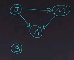
Now we'll continue and we'll add the node A for alarm to the network. And what I want you to do is click on all the other variables that A is dependent on in this network. | |||
[[File:AI class 2011-10-28-205600.PNG]] | |||
{{#ev:youtubehd|X1WygrN9ens}} | |||
The answer is that alarm is dependent on both John and Mary. And so we can draw both nodes in, both arrows in. Intuitively that makes sense because if John calls, then it's more likely that the alarm has occurred, likely as if Mary calls, and if both called, it's really likely. So you can figure out the answer by intuitive reasoning, or you can figure it out by going to the conditional probability tables and seeing according to the definition of conditional probability whether the numbers work out. | |||
{{#ev:youtubehd|rTeQXHTu2_A}} | |||
Now we'll continue and we'll add the node B for burglary, and ask again, click on all the variables that B is dependent on. | |||
[[File:AI class 2011-10-28-210200.PNG]] | |||
{{#ev:youtubehd|_l7rPalYjmU}} | |||
The answer is that B is dependent only on A. In other words, B is independent of J and M given A. | |||
{{#ev:youtubehd|DX1YTIQsjtU}} | |||
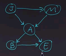
And finally, we'll add the last node, E, and ask you to click on all the nodes that E is dependent on. | |||
{{#ev:youtubehd|T609y-a8bZc}} | |||
And the answer is that E is dependent on A. That much is fairly obvious. But it's also dependent on B. Now, why is that? E is dependent on A because if the earthquake did occur, then it's more likely that the alarm would go off. On the other hand, E is also dependent on B because if a burglary occurred, then that would explain why the alarm is going off, and it would mean that the earthquake is less likely. | |||
[[File:AI class 2011-10-28-210800.PNG]] | |||
== Causal Direction == | |||
{{#ev:youtubehd|YPmGGwlRqY0}} | |||
The moral is that Bayes nets tend to be the most compact and thus the easier to do inference on when they're written in the causal direction -- that is, when the networks flow from causes to effects. | |||
== Variable Elimination == | |||
{{#ev:youtubehd|qyXspkUOhGc}} | |||
Let's return to this equation, which we use to show how to do inference by enumeration. | |||
[[File:AI class 2011-10-28-211200.PNG]] | |||
In this equation, we join up the whole joint distribution before we sum out over the hidden variables. That's slow, because we end up repeating a lot of work. Now we're going to show a new technique called variable elimination, which in many networks operates much faster. It's still a difficult computation, an NP-hard computation, to do inference over Bayes nets in general. Variable elimination works faster than inference by enumeration in most practical cases. It requires an algebra for manipulating factors, which are just names for multidimensional arrays that come out of these probabilistic terms. | |||
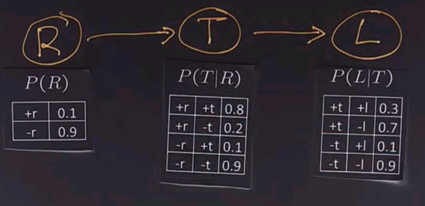
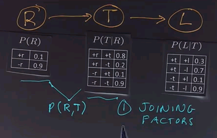
We'll use another example to show how variable elimination works. We'll start off with a network that has three boolean variables. R indicates whether or not it's raining. T indicates whether or not there's traffic, and T is dependent on whether it's raining. And finally, L indicates whether or not I'll be late for my next appointment, and that depends on whether or not there's traffic. | |||
Now we'll put up the conditional probability tables for each of these three variables. | |||
[[File:AI class 2011-10-28-211800.PNG]] | |||
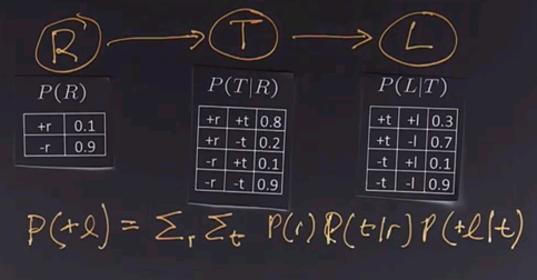
And then we can use inference to figure out the answer to questions like "Am I going to be late?" And we know by definition that we could do that through enumeration by going through all the possible values for R and T and summing up the product of these three nodes. | |||
[[File:AI class 2011-10-28-212000.PNG]] | |||
Now, in a simple network like this, straight enumeration would work fine, but in a more complex network, what variable elimination does is give us a way to combine together parts of the network into smaller parts and then enumerate over those smaller parts and then continue combining. So, we start with a big network. We eliminate some of the variables. We compute by marginalising out, and then we have a smaller network to deal with, and we'll show you how those two steps work. | |||
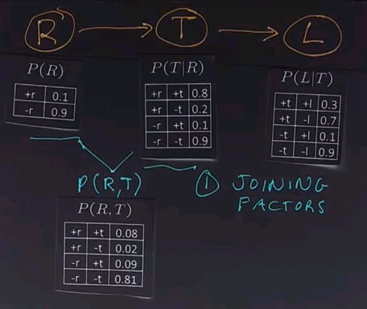
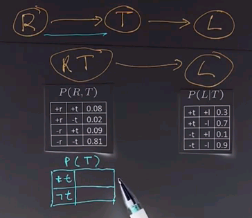
The first operation in variable elimination is called joining factors. A factor, again, is one of these tables. It's a multidimensional matrix, and what we do is choose two of the factors, two or more of the factors. In this case we'll choose these two, and we'll combine them together to form a new factor which represents the joint probability of all the variables in that factor. In this case, R and T. | |||
[[File:AI class 2011-10-28-212600.PNG]] | |||
Now we'll draw out that table. In each case we just look up in the corresponding table, figure out the numbers, and multiply them together. | |||
[[File:AI class 2011-10-28-212800.PNG]] | |||
For example, in this row we have +r and +t, so the +r is 0.1, and the entry for +r and +t is 0.8, so multiply them together and you get 0.08. Go all the way down. For example, in the last row we have a -r and a -t. -r is 0.9. The entry for -r and -t is also 0.9. Multiply those together and you get 0.81. | |||
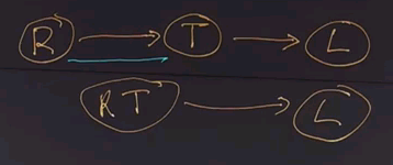
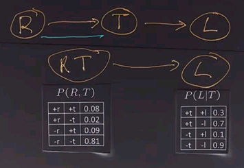
So, what have we done? We used the operation of joining factors on these two factors (R and T), giving us a new factor which is part of the existing network. | |||
[[File:AI class 2011-10-28-213200.PNG]] | |||
Now we want to apply a second operation called elimination, also called summing out or marginalisation, to take this table and reduce it. Right now the tables we have look like this: | |||
[[File:AI class 2011-10-28-213400.PNG]] | |||
We could sum out or marginalise over the variables R to give us a table that just operates on T. So the question is to fill in this table for P(T) -- | |||
[[File:AI class 2011-10-28-213500.PNG]] | |||
there will be two entires in this table, the +t entry formed by summing out all the entries here for all values of r for which t is positive; and the -t entry, formed the same way, by looking in this table and summing up all the rows over all values of r where t is negative. Put your answer in the boxes. | |||
{{#ev:youtubehd|4lm-TI7APX0}} | |||
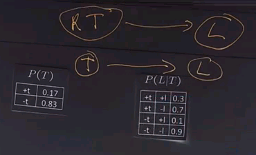
The answer is that for +t we look up the two possible values for r, and we get 0.08 and 0.09. Sum those up, to get 0.17. Then we look at the two possible values of R for -t, and we get 0.02 and 0.81. Add those up, and we get 0.83. | |||
{{#ev:youtubehd|Bk2S3ffdtsc}} | |||
So, we took our network with RT and L. We summed out over R. That gives us a new network with T and L with these conditional probability tables. | |||
[[File:AI class 2011-10-28-214200.PNG]] | |||
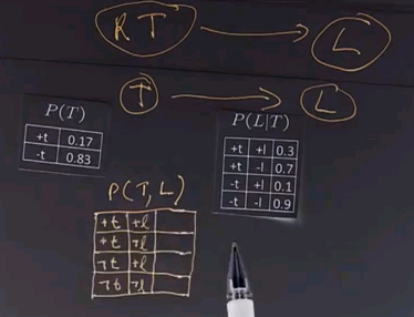
And now we want to do a join over T and L and give us a new table with the joint probability of P(T,L). And that table is going to look like this. | |||
[[File:AI class 2011-10-28-214400.PNG]] | |||
{{#ev:youtubehd|LU9gMODL04Y}} | |||
The answer, again, for joining variables is determined by pointwise multiplication, so we have 0.17 times 0.3 is 0.051, +t and -l, 0.17 times 0.7 is 0.119. Then we go to the minuses. 0.83 times 0.1 is 0.083. And finally, 0.83 times 0.9 is 0.747. | |||
Revision as of 21:00, 28 October 2011
These are my notes for unit 4 of the AI class.
Probabilistic Inference
Overview and Example
{{#ev:youtubehd|1fVWQ-iZqsw}}
Welcome back. In the previous unit, we went over the basics of probability theory and saw how a Bayes network could concisely represent a joint probability distribution, including the representation of independence between the variables. In this unit, we will see how to do probabilistic inference. That is, how to answer probability questions using Bayes nets.
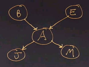
Let's put up a simple Bayes net. We'll use the familiar example of the earthquake where we can have a burglary (B) or an earthquake (E) setting off an alarm (A), and if the alarm goes off, either John (J) or Mary (M) might call.
Now, what kinds of questions can we ask to do inference about? The simplest type of question is the same question we ask with an ordinary subroutine or function in a programming language. Namely, given some inputs, what are the outputs? So, in this case, we could say given the inputs of B and E, what are the outputs J and M?
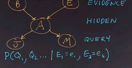
Rather than call them input and output variables, in probabilistic inference, we'll call them evidence and query variables. That is, the variables that we know the values of are the evidence, and the ones that we want to find out the values of are the query variables. Anything that is neither evidence nor query is known as a hidden variable. That is, we won't tell you what its value is. We won't figure out what its value is and report it, but we'll have to compute with it internally.
And now furthermore, in probabilistic inference, the output is not a single number for each of the query variables, but rather it's a probability distribution. So, the answer is going to be a complete, joint probability distribution over the query variables. We call this the posterior distribution, given the evidence, and we can write it like this:
It's the probability distribution of one or more query variables given the values of the evidence variables. And there can be zero or more evidence variables, and each of them are given an exact value. And that's the computation we want to come up with.
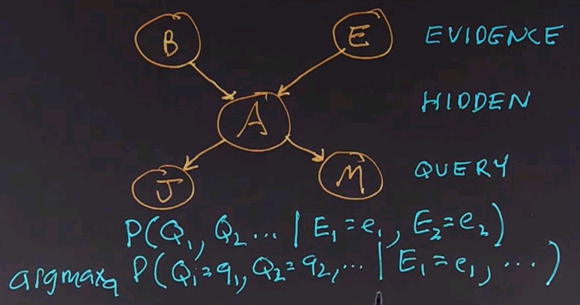
There's another question we can ask. Which is the most likely explanation? That is, out of all the possible values for all the query variables, which combination of values has the highest probability?
We write the formula like this:
asking which Q values are maximal given the evidence values. Now, in an ordinary programming language, each function goes only one way. It has input variables, does some computation, and comes up with a result variable or result variables. One great thing about Bayes nets is that we're not restricted to going only in one direction. We could go in the causal direction, giving as evidence the root nodes of the tree and asking as query values the nodes at the bottom. Or, we could reverse that causal flow. For example, we could have J and M be the evidence variables and B and E be the query variables, or we could have any other combination. For example, we could have M be the evidence variable and J and B be the query variables.
Here's a question for you. Imagine the situation where Mary has called to report that the alarm is going off, and we want to know whether or not there has been a burglary. For each of the nodes, click on the circle to tell us if the node is an evidence node, a hidden node, or a query node.
{{#ev:youtubehd|VYsys0If8bw}}
The answer is that Mary calling is the evidence node. The burglary is the query node, and all the others are hidden variables in this case.
Enumeration
{{#ev:youtubehd|VYsys0If8bw}}
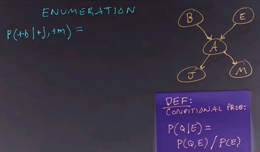
Now we're going to talk about how to do inference on Bayes nets. We'll start with our familiar network, and we'll talk about a method called enumeration, which goes through all the possibilities, adds them up, and comes up with an answer.
So, what we do is start by stating the problem. We're going to ask the question of what is the probability that the burglar alarm occurred given that John called and Mary called? We'll use the definition of conditional probability to answer this.
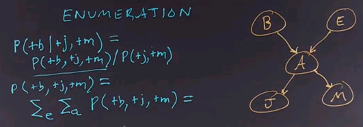
So, this query is equal to the joint probability distribution of all 3 variables divided by the conditionalized variables. Now, note that I'm using a notation here where instead of writing out the probability of some variable equals true, I'm just using the notation plus and then the variable name in lower case, and if I wanted the negation, I would use the negation sign. Notice there's a different notation where instead of writing out the plus and negation signs, we just use the variable name itself, P(e), to indicate E is true.
That notation works well, but it can get confusing between does P(e) mean E is true, or does it mean E is a variable? And so we're going to stick to the notation where we explicitly have the pluses and negation signs.
To do inference by enumeration, we first take a conditional probability and rewrite it as unconditional probabilities. Now we enumerate all the atomic probabilities can calculate the sum of products. Let's look at just the complex term on the numerator first. The procedure for figuring out the denominator would be similar, and we'll skip that.
So, the probability of these three terms together can be determined by enumerating all possible values of the hidden variables. In this case there are 2, E and A. So we'll sum over those variables for all values of E and for all values of A. In this case they're boolean, so there's only two values of each. We ask what's the probability of this unconditional term? And that we get by summing out over all possibilities, E and A being true or false.
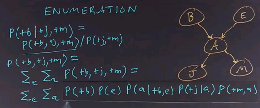
Now, to get the values of these atomic events, we'll have to rewrite this equation in a form that corresponds to the conditional probability tables that we have associated with the Bayes net. So, we'll take this whole expression and rewrite it. It's still a sum over the hidden variables E and A, but now I'll rewrite this expression in terms of the parents of each of the nodes in the network. So, that gives us the product of these five terms, which we then have to sum over all values of E and A.
If we call this product f(e,a), then the whole answer is the sum of F for all values of E and A, so it's the sum of four terms where each of the terms is a product of five numbers.
Where do we get the numbers to fill in this equation?
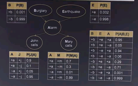
From the conditional probability tables from our model, so let's put the equation back up, and we'll ask you for the case where both E and A are positive to look up in the conditional probability tables and fill in the numbers for each of these five terms, and then multiply them together and fill in the product.
{{#ev:youtubehd|fxYL4PIBXiY}}
We get the answer by reading numbers off the conditional probability tables, so the probability of B being positive is 0.001. Of E being positive, because we're dealing with the positive case now for the variable e, is 0.002. The probability of A being positive, because we're dealing with that case, given that B is positive and the case for an E is positive, that we can read off here as 0.95. The probability that J is positive given that A is positive is 0.9. And finally, the probability that M is positive given that A is positive we read off here as 0.7. We multiply all those together, it's going to be a small number because we've got the 0.001 and the 0.002 here. Can't quite fit it in the box, but it works out to 0.000001197. That seems like a really small number, but remember, we have to normalize by the P(+j,+m) term, and this is only one of the four possibilities. We have to enumerate over all four possibilities for E and A, and in the end, it works out that the probability of the burglar alarm being true given that John and Mary calls, is 0.284.
And we get that number because, intuitively, it seems that the alarm is fairly reliable, John and Mary calling are very reliable, but the prior probability of burglary is low. And those two terms combine together to give us the 0.284 value when we sum up each of the four terms of these products.
Speeding Up Enumeration
{{#ev:youtubehd|DWO-XKo2iS8}}
We've seen how to do enumeration to solve the inference problem on belief networks. For a simple network like the alarm network, that's all we need to know. There's only five variables, so even if all five of them were hidden, there would only be 32 rows in the table to sum up. From a theoretical point of view, we're done. But from a practical point of view, other networks could give us trouble. Consider this network, which is one for determining insurance for car owners. There are 27 difference variables. If each of the variables were boolean, that would give us over 100 million rows to rum out. But in fact, some of the variables are non-boolean, they have multiple values, and it turns out that representing this entire network and doing enumeration we'd have to sum over a quadrillion rows. That's just not practical, so we're going to have to come up with methods that are faster than enumerating everything.
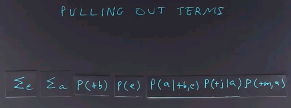
The first technique we can use to get a speed-up in doing inference on Bayes nets is to pull out terms from the enumeration.
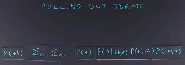
For example, here the probability of B is going to be the same for all values of E and A. So we can take that term and move it out of the summation, and now we have a little bit less work to do.
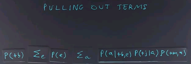
We can multiply by that term once rather than having it in each row of the table. We can also more this term, P(e), to the left of the summation over a, because it doesn't depend on a.
By doing this, we're doing less work. The inner loop of the summation now has only three terms rather than five terms. So we've reduced the cost of doing each row of the table. But we still have the same number of rows in the table, so we're gonna have to do better than that.
The next technique for efficient inference is to maximise the independence of variables. The structure of a Bayes net determines how efficient it is to do inference on it. For example, a network that's a linear string of variables, X1 through Xn, can have inference done in time proportional to the number n,
whereas a network that's a complete network where every node points to every other node and so on could take time 2n if all n variables are boolean variables.
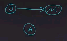
In the alarm network we saw previously, we took care to make sure that we had all the independence relations represented in the structure of the network. But if we put the nodes together in a different order, we would end up with a different structure. Let's start by ordering the node "John calls" first. And then adding the node "Mary calls". The question is, given just these two nodes and looking at the node for "Mary calls", is that node dependent or independent of the node for "John calls"?
{{#ev:youtubehd|r3mOvkvHbts}}
The answer is that the node for "Mary calls" in this network is dependent on "John calls". In the previous network, they were independent given that we know that the alarm had occurred. But here we don't know that the alarm had occurred, and so the nodes are dependent because having information about one will affect the information about the other.
{{#ev:youtubehd|uZfGhIFH92g}}
Now we'll continue and we'll add the node A for alarm to the network. And what I want you to do is click on all the other variables that A is dependent on in this network.
{{#ev:youtubehd|X1WygrN9ens}}
The answer is that alarm is dependent on both John and Mary. And so we can draw both nodes in, both arrows in. Intuitively that makes sense because if John calls, then it's more likely that the alarm has occurred, likely as if Mary calls, and if both called, it's really likely. So you can figure out the answer by intuitive reasoning, or you can figure it out by going to the conditional probability tables and seeing according to the definition of conditional probability whether the numbers work out.
{{#ev:youtubehd|rTeQXHTu2_A}}
Now we'll continue and we'll add the node B for burglary, and ask again, click on all the variables that B is dependent on.
{{#ev:youtubehd|_l7rPalYjmU}}
The answer is that B is dependent only on A. In other words, B is independent of J and M given A.
{{#ev:youtubehd|DX1YTIQsjtU}}
And finally, we'll add the last node, E, and ask you to click on all the nodes that E is dependent on.
{{#ev:youtubehd|T609y-a8bZc}}
And the answer is that E is dependent on A. That much is fairly obvious. But it's also dependent on B. Now, why is that? E is dependent on A because if the earthquake did occur, then it's more likely that the alarm would go off. On the other hand, E is also dependent on B because if a burglary occurred, then that would explain why the alarm is going off, and it would mean that the earthquake is less likely.
Causal Direction
{{#ev:youtubehd|YPmGGwlRqY0}}
The moral is that Bayes nets tend to be the most compact and thus the easier to do inference on when they're written in the causal direction -- that is, when the networks flow from causes to effects.
Variable Elimination
{{#ev:youtubehd|qyXspkUOhGc}}
Let's return to this equation, which we use to show how to do inference by enumeration.
In this equation, we join up the whole joint distribution before we sum out over the hidden variables. That's slow, because we end up repeating a lot of work. Now we're going to show a new technique called variable elimination, which in many networks operates much faster. It's still a difficult computation, an NP-hard computation, to do inference over Bayes nets in general. Variable elimination works faster than inference by enumeration in most practical cases. It requires an algebra for manipulating factors, which are just names for multidimensional arrays that come out of these probabilistic terms.
We'll use another example to show how variable elimination works. We'll start off with a network that has three boolean variables. R indicates whether or not it's raining. T indicates whether or not there's traffic, and T is dependent on whether it's raining. And finally, L indicates whether or not I'll be late for my next appointment, and that depends on whether or not there's traffic.
Now we'll put up the conditional probability tables for each of these three variables.
And then we can use inference to figure out the answer to questions like "Am I going to be late?" And we know by definition that we could do that through enumeration by going through all the possible values for R and T and summing up the product of these three nodes.
Now, in a simple network like this, straight enumeration would work fine, but in a more complex network, what variable elimination does is give us a way to combine together parts of the network into smaller parts and then enumerate over those smaller parts and then continue combining. So, we start with a big network. We eliminate some of the variables. We compute by marginalising out, and then we have a smaller network to deal with, and we'll show you how those two steps work.
The first operation in variable elimination is called joining factors. A factor, again, is one of these tables. It's a multidimensional matrix, and what we do is choose two of the factors, two or more of the factors. In this case we'll choose these two, and we'll combine them together to form a new factor which represents the joint probability of all the variables in that factor. In this case, R and T.
Now we'll draw out that table. In each case we just look up in the corresponding table, figure out the numbers, and multiply them together.
For example, in this row we have +r and +t, so the +r is 0.1, and the entry for +r and +t is 0.8, so multiply them together and you get 0.08. Go all the way down. For example, in the last row we have a -r and a -t. -r is 0.9. The entry for -r and -t is also 0.9. Multiply those together and you get 0.81.
So, what have we done? We used the operation of joining factors on these two factors (R and T), giving us a new factor which is part of the existing network.
Now we want to apply a second operation called elimination, also called summing out or marginalisation, to take this table and reduce it. Right now the tables we have look like this:
We could sum out or marginalise over the variables R to give us a table that just operates on T. So the question is to fill in this table for P(T) --
there will be two entires in this table, the +t entry formed by summing out all the entries here for all values of r for which t is positive; and the -t entry, formed the same way, by looking in this table and summing up all the rows over all values of r where t is negative. Put your answer in the boxes.
{{#ev:youtubehd|4lm-TI7APX0}}
The answer is that for +t we look up the two possible values for r, and we get 0.08 and 0.09. Sum those up, to get 0.17. Then we look at the two possible values of R for -t, and we get 0.02 and 0.81. Add those up, and we get 0.83.
{{#ev:youtubehd|Bk2S3ffdtsc}}
So, we took our network with RT and L. We summed out over R. That gives us a new network with T and L with these conditional probability tables.
And now we want to do a join over T and L and give us a new table with the joint probability of P(T,L). And that table is going to look like this.
{{#ev:youtubehd|LU9gMODL04Y}}
The answer, again, for joining variables is determined by pointwise multiplication, so we have 0.17 times 0.3 is 0.051, +t and -l, 0.17 times 0.7 is 0.119. Then we go to the minuses. 0.83 times 0.1 is 0.083. And finally, 0.83 times 0.9 is 0.747.
