AI class unit 3
These are my notes for unit 3 of the AI class.
Probability in AI
Introduction
So the next units will be concerned with probabilities. Particularly with structured probabilities using Bayes Networks. This is some of the most involved material in this class. And since this is a Stanford level class you'll find out that some of the quizzes are actually real hard. So as you go through the material I hope the hardness of the quizzes won't discourage you, it'll really entice you, to take a piece of paper and a pen and work them out.
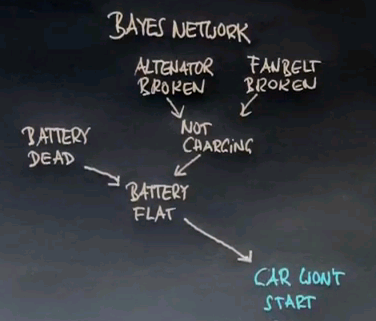
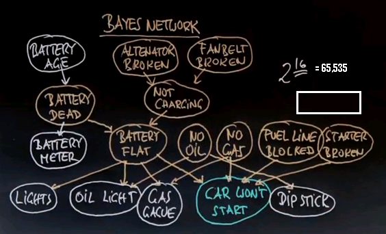
Let me give you a flavour of a Bayes Network using an example. Suppose you find in the morning that your car won't start. Well there are many causes why your car might not start. One is that your battery is flat. Even for a flat battery there's multiple causes: one is that it's just plain dead, and one is that the battery is OK but it's not charging. The reason why a battery might not charge is that the alternator may be broken or the fan belt may be broken. If you look at this influence diagram, also called a Bayes Network, you'd find that there's many different ways to explain that the car won't start, and a natural question you might have is "can we diagnose the problem?"
One diagnostic tool is a battery meter, which may increase or decrease your belief that the battery may cause you car failure. You might also know your battery age -- older batteries tend to go dead more often. Then there's many other ways to look at reasons why the car won't start. You might expect the lights, the oil light, the gas gauge. You might even dip into the engine to see what the oil level is, with a dipstick. And all of those relate to alternative reasons why your car might not be starting, like no oil, or no gas, the fuel line might be blocked, or the starter might be broken. All of these can influence your measurements, like the oil light or the gas gauge, in different ways. For example a flat battery might have an effect on the lights, or the oil light, and on the gas gauge; but it won't really have an effect the oil you measure with a dipstick. That is affected by the oil level, which also affects the oil light. Gas will affect the gas gauge and of course without gas the car doesn't start.
So this is a complicated structure that really describes one way to understand how a car doesn't start. A car is a complex system, it has lots of variables you can't really measure immediately, and it has sensors which allow you to understand a little bit about the state of the car.
What the Bayes Network does, is it really assists you in reasoning from observable variables like the car won't start and the value of the dipstick to hidden causes like is the fan belt broken or is the battery dead? What we have here is a Bayes Network. A Bayes Network is composed of nodes, these nodes correspond to events that you might or might not know, they're typically called random variables. These nodes are linked by arcs and the arcs suggest that a child of an arc is influenced by its parent, but not in a deterministic way it might be influenced in a probabilistic way. Which means an older battery for example has a higher chance of causing the battery to be dead, but it's not clear that every old battery is dead.
There's a total of 16 variables in this Bayes Network. What the graph structure and associated probabilities specify is a huge probability distribution in the space of all of these 16 variables. If they were binary, which we'll assume throughout this unit, they can take 216 different values, which is a lot.
The Bayes Network as we'll find out is a compact representation of a distribution over this very very large joint probability distribution of all of these variables. Further, once we've specified the Bayes Network we can observe for example that the car won't start, you can observe things like the oil light, and the lights and the battery and then compute probabilities of hypotheses like the alternator is broken, or the fan belt is broken, or the battery is dead. So in this class we're going to talk about how to construct these Bayes Networks, what the semantics are, and how to reason in this Bayes Network to find out about variables we can't observe like whether the fan belt is broken or not.
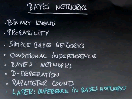
That's an overview. Throughout this unit we are going to assume that every event is discrete, in fact it's binary. We'll start with some consideration of basic probability. We'll work our way into some simpler Bayes Networks. We'll talk about concepts like conditional independence. Then we'll define Bayes Network more generally. Move into a concept like D-separation, and start doing parameter counts. Later on Peter will tell you about inference in Bayes Networks, so we won't be doing that in this class.
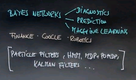
I can't overemphasise how important this class is. Bayes Networks are used extensively in almost all fields of smart computer systems. In diagnostics, for prediction, for machine learning. In fields like finance, inside Google, in robotics.
Bayes Networks are also the building blocks of more advanced AI techniques such as particle filters, Hidden Markov Models, MDPs and POMDPs, Kalman filters, and many others. These are words that don't sound familiar quite yet but as you go through the class I can promise you that you will get to know what they mean.
So let's start now with the very very basics.
Probability/Coin Flip
So let's talk about probabilities. Probabilities are the corner stone of artificial intelligence. They are used to express uncertainty, and the management of uncertainty is really key to many many things in AI such as machines learning and Bayes Network inference and filtering and robotics and computer vision and so on.
So we're going to start with some very basic questions and we're going to work our way out from there.
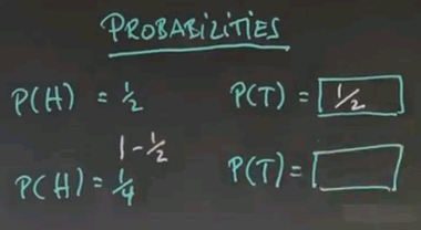
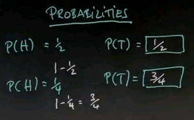
Here's a coin, and the coin came up heads or tails. And my question is the following: suppose the probability for heads is 0.5 what's the probability for it coming up tails?
So the right answer is a half, or 0.5, and the reason is that the coin can only come up heads or tails, we know that it has to be either one, therefore the total probability of both coming up is one. So half the probability is assigned to heads, and the other half is assigned to tails.
Let me ask the next quiz. Suppose the probability of heads is a quarter, 0.25, what is the probability of tails?
And the answer is three quarters, it's a loaded coin and the reason is, well, each of them has a certain probability. The total of those is one. The quarter is claimed by heads. Therefore, 3/4 remain for tail, which is the answer over here.
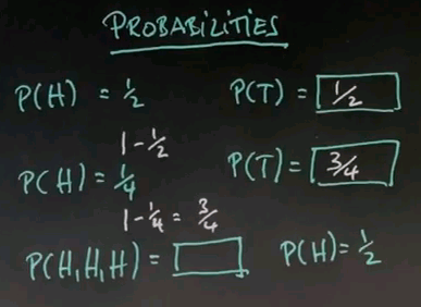
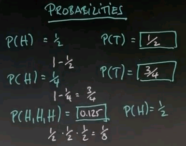
Here's another quiz. What's the probability that the coin comes up heads, heads, heads, three times in a row, assuming that each one of those has a probability of a half and that these coin flips are independent.
The answer is 0.125. Each head has a probability of a half. We can multiply those probabilities because they are independent events. And that gives us 1/8 or 0.125.
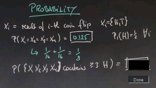
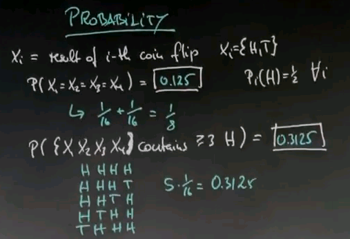
Now let's flip the coin four times, and let's call Xi the result of the i-th coin flip. So each Xi is going to be drawn from heads (H) or tails (T). What's the probability that all four of those flips give us the same result, no matter what it is, assuming that each one of those has identically and an equally distributed probability of coming up heads of a half.
And the answer is, well, there's 2 ways that we can achieve this. One is the all heads and one is all tails. You already know that 4 times heads is 1/16, and we know that 4 times tails is also 1/16. These are completely independent events. The probability of either one occurring is 1/16 plus 1/16, which is 1/8, which is 0.125.
So here's another one. What's the probability that within the set of X1, X2, X3 and X4 there are at least three (or more) heads?
And the solution is let's look at different sequences in which heads occurs at least 3 times. It could be head, head, head, head, in which it comes 4 times. It could be head, head, head, tail and so on, all the way to tail, head, head, head. There is 1, 2, 3, 4, 5 of those outcomes. Each of them has a 16th for probability, so it's 5 times a 16th, which is 0.3125.
Probability Summary
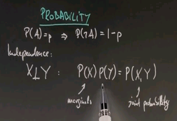
So we just learned a number of things. One is about complementary probability. If an event has a certain probability, P, then the complementary event has probability 1-P. We also learned about independence. If 2 random variables, X and Y, are independent, which you're going to write as shown below, that means the probability of the joint that any 2 variables can assume is the product of the marginals. So rather than asking the question, "What is the probability for any combination that these 2 coins or maybe 5 coins could have taken?" we can now look at the probability of each coin individually, look at its probability and just multiply them up.
Dependence
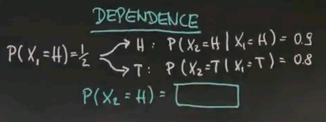
So let me ask you about dependence. Suppose we flip 2 coins. Our first coin is a fair coin, and we're going to denote the outcome by Xi. So the chance of X1 coming up heads is half. But now we branch into picking a coin based on the first outcome. So if the first outcome was heads, you pick a coin whose probability of coming up heads is going to be 0.9. The way I word this is by conditional probability, the probability of the second coin flip coming up heads provided that, or given that, X1, the first coin flip, was heads, is 0.9. The first coin flip might also come up tails, in which case I pick a very different coin. In this case I pick a coin which with 0.8 probability will once again give me tails, conditioned on the first coin flip coming up tails. So my question for you is, what's the probability of the second coin flip coming up heads?
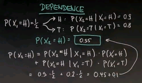
The answer is 0.55. The way to compute this is by the theorem of total probability. The probability of X2 equals heads. There's two ways I can get into this outcome. One is via this path over here, and one is via this path over here. Let me just write both of them down.
So first of all, it could be the probability of X2 equals heads given that, and I will assume, X1 was heads already. Now I have to add the complementary event. Suppose X1 came up tails. Then I can ask the question, what is the probability that X2 comes up heads regardless, even though X1 was tails.
Plugging the numbers gives us the following. This one over here is 0.9 times a half. The probability of tails is 0.8 thereby my heads probability becomes 1 minus 0.8, which is 0.2. Adding all this together gives me 0.45 plus 0.1, which is exactly 0.55.
What We Learned
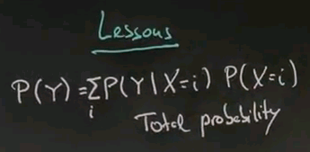
So, we actually just learned some interesting lessons. The probability of any random variable Y can be written as the probability of Y given that some other random variable X assumes value i times the probability of X equals i, summed over all possible outcomes i for the random variable X. This is called total probability.
The second thing we learned has to do with negation of probabilities. We found that probability of not X given Y is 1 minus probability of X given Y. Now, you might be tempted to say "What about the probability of X given not Y?" "Is this the same as 1 minus probability of X given Y?" And the answer is absolutely no. That's not the case. If you condition on something that has certain probability value, you can take the event you're looking at and negate this, but you can never negate your conditional variable and assume these values add up to 1.
Weather
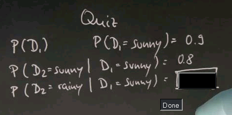
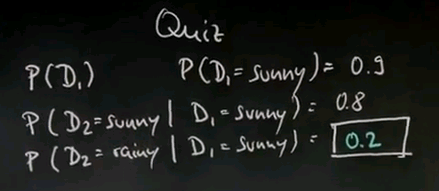
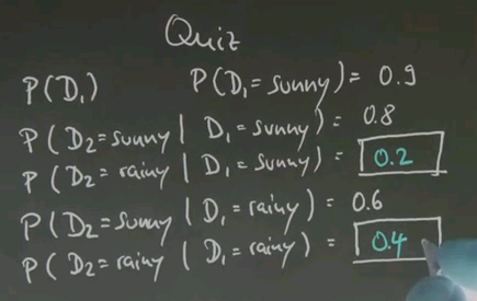
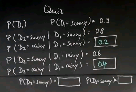
We assume there is sometimes sunny days and sometimes rainy days, and on day 1, which we're going to call D1, the probability of sunny is 0.9. And then let's assume that a sunny day follows a sunny day with 0.8 chance, and a rainy day follows a sunny day with, well?
Well, the correct answer is 0.2, which is a negation of this event over here.
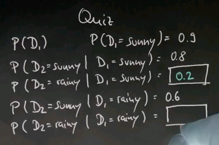
A sunny day follows a rainy day with 0.6 chance, and a rainy day follows a rainy day with: please give me your number.
So, what are the chances that D2 is sunny? Suppose the same dynamics apply from D2 to D3, so just replace D3 over here with D2s over there. That means the transition probabilities from one day to the next remain the same. Tell me, what's the probability that D3 is sunny?
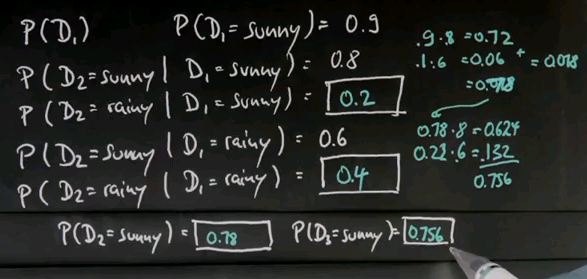
So, the corrent answer for P(D2=sunny) is 0.78, and for P(D3=sunny) it's 0.756. To get there, let's complete P(D2=sunny) first. The probability of D2 = sunny. Well, we know there's a 0.9 change it's sunny on D1, and then if it is sunny, we know it stays sunny with a 0.8 chance. So, we multiply P(D1=sunny) (0.9) and P(D2=sunny | D1=sunny) (0.8) together, and we get 0.72. We know there's a 0.1 chance of it being rainy on day 1, which is the complement, but if it's rainy, we know it switches to sunny with 0.6 change, so you multiply P(D1=rainy) and P(D2=sunny | D1=rainy), and you get 0.06. Adding those two results up equals 0.78.
Now, for the next day, we know our prior for sunny is 0.78. If it is sunny, it stays sunny with 0.8 probability. Multiplying these two things gives us 0.624. We know it's rainy with 0.22 chance, which is the complement of 0.78, but a 0.6 chance if it was sunny. If you multiply those it's 0.132. Adding those two things up gives us 0.756.
So to some extent it's tedious to compute these values, but they can be perfectly computed, as shown here.
Cancer
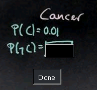
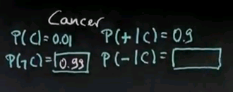
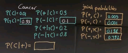
The next example is a cancer example. Suppose there is a specific type of cancer that exists for 1% of the population. That will be written as follows. You can probably tell me now what the probability of not having cancer is?
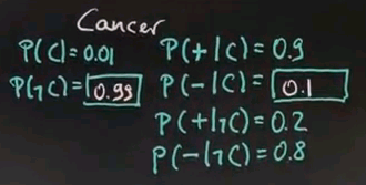
And yes, the answer is 0.99. Let's assume there's a test for this cancer, which gives us probabilistically an answer whether we have this cancer or not. So, let's say the probability of a test being positive, as indicated by this + sign, given that we have the cancer is 0.9. The probability of the test coming out negative if we have the cancer is..?
The answer is 0.1, which is the difference between 1 and 0.9. Let's assume the probability of the test coming out positive given that we don't have this cancer is 0.2. In other words, the probability of the test correctly saying we don't have he cancer if we're cancer free is 0.8.
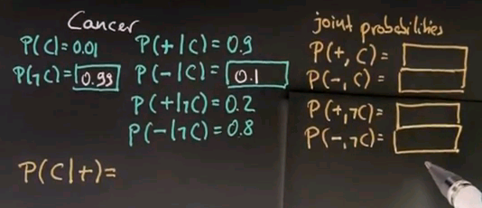
Now, ultimately, I'd like to know what's the probability they have this cancer given they just received a single, positive test? Before I do this, please help me filling out some other probabilities that are actually important. Specifically, the joint probabilities. The probability of a positive test and having cancer. The probability of a negative test and having cancer, and this is not conditional any more. It's now a joint probability. So, please give me those four values over here:
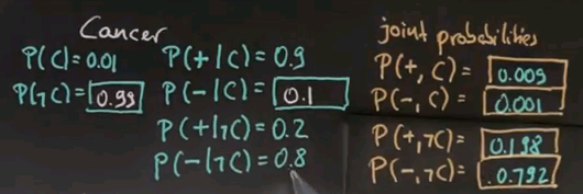
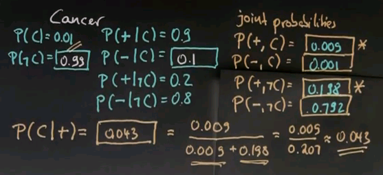
And here are the correct answers. 0.009, which is the product of your prior, 0.01, times the conditional, 0.9. Next we get 0.001, the probability of our prior cancer time 0.1. Then we get 0.198, the probability of not having cancer is 0.99 times still getting a positive reading, which is 0.2. And finally we get 0.792, which is the probability of P(-,~C) times P(~C).
Now, our next quiz, I want you to fill in the probability of having cancer given that we just received a positive test.
And the correct answer is 0.043. So, even though I received a positive test, my probability of having cancer is just 4.3%, which is not very much given that the test itself is quite sensitive. It really gives me a 0.8 chance of getting a negative result if I don't have cancer. It gives me a 0.9 chance of detecting cancer given that I have cancer.
Now, what comes out is small. Well, let's just put all the cases together. You already know that we received a positive test. Therefore, the entry P(+,C), and the entry P(+,~C) are relevant. Now, the chance of having a positive test and having cancer is 0.009. Well, I might -- when I receive a positive test -- have cancer or not cancer, so we will just normalize by these 2 possible causes for the positive test, which is 0.009 + 0.198. We now put these 2 things together and get 0.009 over 0.207. Which is approximately 0.043.
Now, the interesting thing in this equation is that the chances of having seen a positive test result in the absence of cancers are still much much higher than the chance of seeing a positive result in the presence of cancer, and that's because our prior for cancer is so small in the population that it's just very unlikely to have cancer. So, the additional information of a positive test only raised by posterior probability to 0.043.
See this question on Aiqus for another explanation of the working.
Bayes Rule
So, we've just learned about what's probably the most important piece of math for this class in statistics called Bayes Rule. It was invented by Reverend Thomas Bayes, who was a British mathematician and a Presbyterian minister in the 18th century.
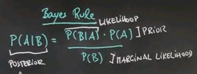
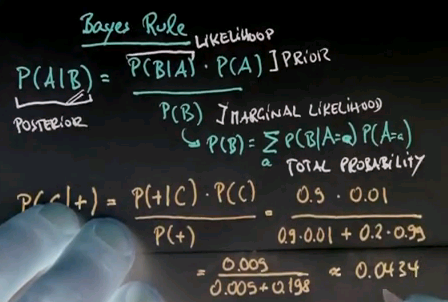
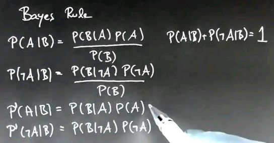
Bayes Rule is usually stated as follows: P of A given B where B is the evidence and A is the variable we care about is P of B given A times P of A over P of B.
P(A|B) = P(B|A) P(A) / P(B)
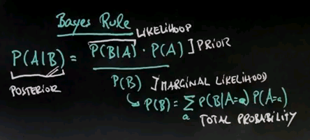
P(B|A) is called the likelihood. P(A) is called the prior. P(B) is called the marginal likelihood. P(A|B) is called the posterior.
The interesting thing here is the way the probabilities are reworded. Say we have evidence B. We know about B, but we really care about the variable A. So, for example, B is a test result. We don't care about the test result as much as we care about the fact whether we have cancer or not.
This diagnostic reasoning -- which is from evidence to its causes -- is turned upside down by Bayes Rule into causal reasoning, which is given. Hypothetically if we knew the cause what would be the probability of the evidence we just observed. But to correct for this inversion, we have to multiply by the prior of the cause to be the case in the first place, in this case having cancer or not, and divide it by the probability of the evidence, P(B), which often is expanded using the theorem of total probability as follows.
The probability of B is a sum over all probabilities of B conditional on A, low caps a, times the probability of A equals lower caps a. This is total probability as we already encountered it.
So, let's apply this to the cancer case and say we really care about whether you have cancer, which is our cause, conditioned on the evidence that is the result of this hidden cause, in this case, a positive test result. Let's just plug in the numbers. Our likelihood is the probability of seeing a positive test result given that you have cancer multiplied by the prior probability of having cancer over the probability of the positive test result, and that is -- according to the tables we looked at before -- 0.9 times a prior of 0.01 over -- now we're going to expand this right over here according to the total probability which gives us 0.9 times 0.01. That's the probability of + given that we do have cancer. So, the probability of + given that we don't have cancer is 0.2, but the prior here is 0.99.
So, if we plug in the numbers we know about, we get 0.009 over 0.009 + 0.198. That is approximately 0.0434, which is the number we saw before.
Bayes Network
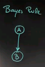
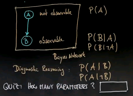
So if you want to draw Bayes Rule graphically we have a situation where we have an internal variable A, like whether or not we have cancer, but we can't sense A. Instead, we have a second variable, called B, which is our test, and B is observable, but A isn't.
This is a classical example of a Bayes network. The Bayes network is composed of 2 variables, A and B. We know the prior probability for A, and we know the conditional. A causes B -- whether or not we have cancer, causes the test result to be positive or not, although there was some randomness involved. So, we know what the probability of B given the different values for A, and what we care about in this specific instance is called diagnostic reasoning, which is the inverse of the causal reasoning, the probability of A given B or similarly, probability of A given not B.
This is our very first Bayes network, and the graphical representation of drawing two variables, A and B, connected with an arc that goes from A to B is the graphical representation of a distribution of two variables that are specified in the structure, which has a prior probability and has a conditional probability as shown.
Now I do have a quick quiz for you. How many parameters does it take to specify the entire joint probability within A and B, or dirrently, the entire Bayes network?
I'm not looking for structural parameters that relate to the graph over here. I'm just looking for the numerical parameters of the underlying probabilities.
And the answer is three. It takes 1 parameter to specify P(A) from which we can derive P(~A). It takes 2 parameters to specify P(B|A) and P(B|~A), from which we can derive P(~B|A) and P(~B|~A).
So it's a total of 3 parameters for this Bayes network.
Computing Bayes Rule
So, we just encountered our very first Bayes network and did a number of interesting calculations. Let's now talk about Bayes Rule and look into more complex Bayes networks.
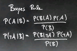
I will look at Bayes Rule again and make an observation that is really non-trivial. Here's Bayes Rule, and in practice, what we find is P(B|A)P(A) is relatively easy to compute. It's just a product, whereas P(B) is really hard to compute. However, P(B) does not depend on what we assume for variable A, it's just a function of B.
So, suppose for a moment we also care about the complementary event P(~A|B) for which Bayes Rule unfolds as follows. Then we find that the normalizer, P(B), is identical, whether we assume A on the left side or ~A on the left side.
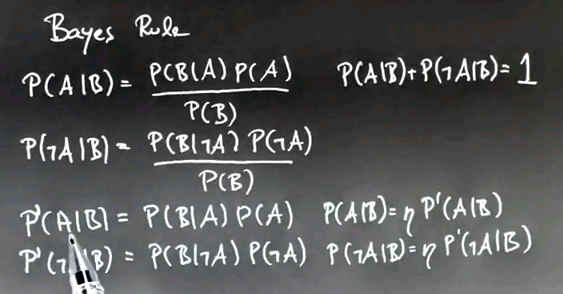
We also know from prior work that P(A|B) plus P(~A|B) must be one because these are 2 complementary events. That allows us to compute Bayes Rule very differently by basically ignoring the normalizer, so here's how it goes:
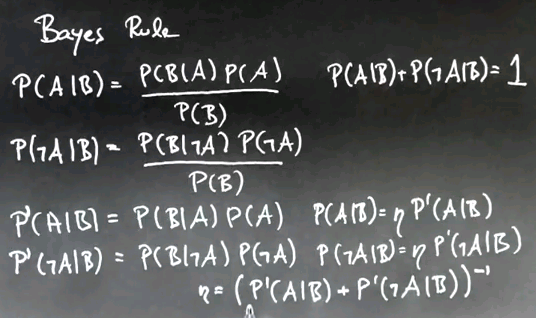
We compute P'(A|B) -- and I want to call this prime, because it's not a real probability -- to be just P(B|A)P(A), which is the normalizer, so the denominator of the expression over here. We do the same thing with P'(~A|B).
So, in both cases, we compute the posterior probability non-normalized by omitting the normalizer P(B). And then we can recover the original probabilities by normalizing based on P'(A|B) and P'(~A|B), so the probability of P(A|B), the actual probability, is a normalizer, eta, times this non-normalized form P'(A|B).
The same is true for the negation P(~A|B). And eta is just the normalizer that results by adding the two values for P'(A|B) + P'(~A|B) together and dividing them for one.
So, take a look at this for a moment. What we've done is we deferred the calculation of the normalizer by computing pseudo probabilities that are non-normalized. This made the calculation much easier, and when we were done with everything, we just folded back in the normalizer base on the resulting pseudo probabilities and got the correct answer.
Two Test Cancer
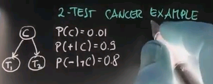
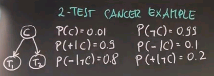
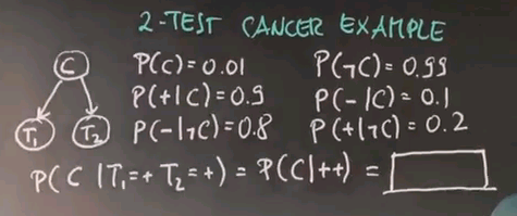
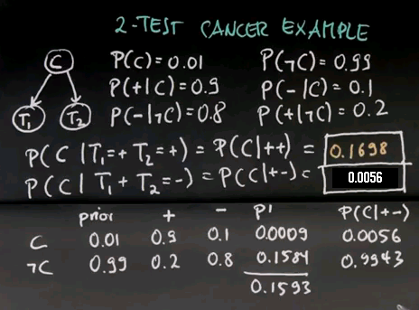
The reason why I gave you all this is because I want you to apply it now to a slightly more complicated problem, which is the 2-test cancer example. In this example, we again might have our unobservable cancer C, but now we're running two tests, test 1 and test 2. As before, the prior probability of cancer is 0.01. The probability of receiving a positive test result for either test is 0.9. The probability of getting a negative result given they're cancer free is 0.8.
And from those we were able to compute all the other probabilities, and we're just going to write them down over here.
So, take a moment to just verify those. Now, let's assume both of my tests come back positive, so T1=+ and T2=+. What's the probability of cancer now written in short for probability of P(C|++)? I want you to tell me what that is, and this is a non-trivial question.
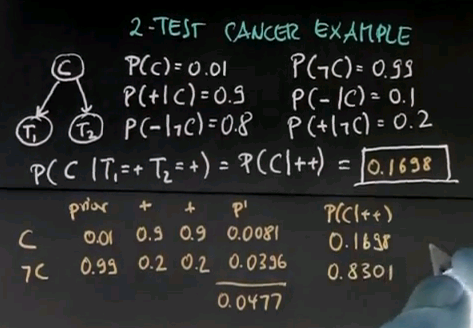
So, the correct answer is 0.1698 approximately, and to compute this, I used the trick I've shown you before. Let me write down the running count for cancer and for not cancer as I integrate the various multiplications in Bayes Rule. My prior for cancer was 0.01 and for non-cancer was 0.99. Then I get my first +, and the probability of a + given they have cancer is 0.9, and the same for non-cancer is 0.2. So, according to the non-normalized Bayes Rule, I now multiply these 2 things together to get my non-normalized probability of having cancer given the +. Since multiplication is commutative I can do the same thing again with my 2nd test result, 0.9 and 0.2, and I multiply all of these 3 things together to get my non-normalized probability P' (P prime) to be the following: 0.0081, if you multiply the top row together, and 0.0396 if you multiply the bottom row together. And these are not a probability. If we add those for the 2 complementary of cancer and non-cancer, we get 0.0477. However, if I now divide, that is, I normalize those non-normalized probabilities over here by this factor over here, I actually get the correct posterior probability P(C|++). And they look as follows: approximately 0.1698 and approximately 0.8301.
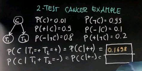
Calculate for me the probability of cancer given that I received one positive and one negative test result. Please write your number into this box.
We apply the same trick as before where we use the exact same prior of 0.01. Our first + gives us the following factors: 0.9 and 0.2. And our minus gives us the probability 0.1 for a negative first test result given that we have cancer, and a 0.8 for the inverse of a negative result of not having cancer. We multiply those together and we get our non-normalized probability. And if we now normalize by the sum of those two things, to turn this back into a probability, we get 0.009 over the sum of those two things here, and this is 0.0056 for the chance of having cancer and 0.9943 for the chance of being cancer free.
Conditional Independence
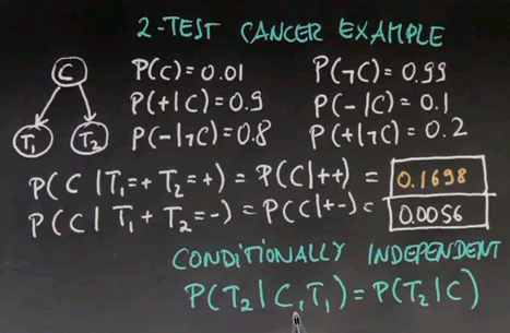
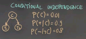
I want to use a few words of terminology. This, again, is a Bayes network, of which the hidden variable C causes the still stochastic test outcomes T1 and T2. And what's really important is that we assume not just that T1 and T2 are identically distributed. We use the same 0.9 for test 1 as we use for test 2, but we also assume that they are conditionally independent. We assumed that if God told us whether we actually had cancer or not, if we knew with absolute certainty the value of the variable C, that knowing anything about T1 would not help us make a statement about T2.
Put differently, we assumed that the probability of T2 given C and T1 is the same as the probability of T2 given C. This is called conditional independence, which is given the value of the cancer variable C. If you knew this for a fact, then T2 would be independent of T1. It's conditionally independent because the independence only holds true if we actually know C, and it comes out of this diagram over here (the network in the top left).
If we look at this diagram (the Bayes network), if you know the variable C over here, then C separately causes T1 and T2. So, as a result, if you know C, whatever counted over here is kind of cut off casually from what happens over here. That causes these 2 variables to be conditionally independent. So, conditional independence is a really big thing in Bayes networks.
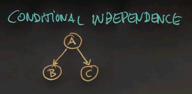
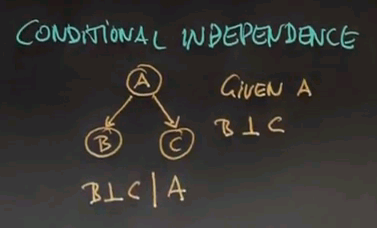
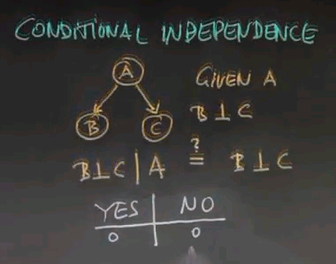
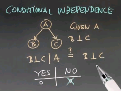
Here's a Bayes network where A causes B and C, and for a Bayes network of this structure, we know that given A, B and C are independent. It's written as B conditionally independent of C given A,
So here's a question: Suppose we have conditional independence between B and C given A. Would that imply -- and there's my question -- that B and C are independent? So, suppose we don't know A. We don't know whether we have cancer, for example. What that means is that the test results individually are still independent of each other even if we don't know about the cancer situation. Please answer yes or no.
And the correct answer is No. Intuitively, getting a positive test result about cancer gives us information about whether you have cancer or not. So if you get a positive test result you're going to raise the probability of having cancer relative to the prior probability. With that increased probability we will predict that another test will with a higher likelihood give us a positive response that if we hadn't taken the previous test. That's really important to understand. So that we understand it let me make you calculate those probabilities.
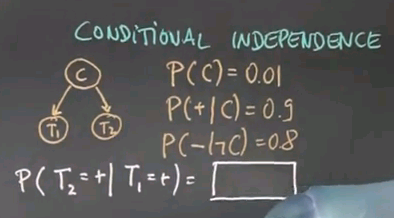
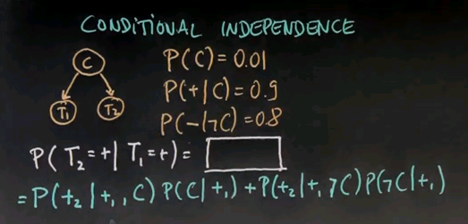
Let me draw the cancer example again with two tests. Here's my cancer variable and then there's two conditionally independent tests T1 and T2. And as before let me assume that the prior probability of cancer is 0.01.
What I want you to compute for me is the probability of the second test to be positive if we know that the first test was positive. So write this into the following box.
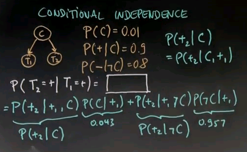
So, for this one, we want to apply total probability. This thing over here is the same as probability of T2 to be positive, which I'm going to abbreviate with a +2 over here, conditioned on T1 being positive and me having cancer times the probability of me having cancer given T1 was positive plus the probability of T2 being positive conditioned on T1 being positive and me not having cancer time the probability of me not having cancer given that T1 is positive.
That's the same as the theorem of total probability, but now everything is conditioned on +1. Take a moment to verify this.
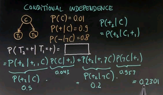
Now, here I can plug in the numbers. You already calculated this one (P(C|+1)) before, which is approximately 0.043, and this one over here (P(~C|+1)) is 1 minus that, which is 0.957 approximately. And this term over here (P(+2|+1,C)) now exploits conditional independence, which is given that I know C, knowledge of the first test gives me no more information about the second test. It only gives me information if C was unknown, as was the case over here.
So, I can rewrite this thing over here (P(+2|+1,C)) as follows:
P(+2|C). I can drop the +1, and the same is true over here (P(+2|+1,~C)). This is exploiting my conditional independence.
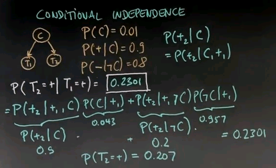
I knew that P(+2|C) = P(+2|C,+1. I can now read those off my table over here, which is 0.9 times 0.043 plus 0.2 -- which is 1 minus 0.8 over here (P(-|~C)) -- times 0.957, which gives me approximately 0.2301.
So, that says if my first test comes in positive, I expect my second test to be positive with probability 0.2301. That's an increased probability to the default probability, which we calculated before, which is the probability of any test, test 2 come in as positive before was (inaudible) of Bayes rule which was 0.207.
So, my first test has a 20% chance of coming in positive. My second test, after seeing a positive test, has now an increased probability of about 23% of coming in positive.
Absolute and Conditional
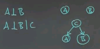
So, now we've learned about independence, and the corresponding Bayes network has 2 nodes. They're just not connected at all. And we learned about conditional independence in which case we have a Bayes network that looks like this:
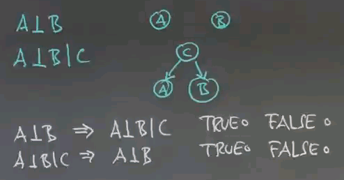
Now I would like to know whether absolute independence implies conditional independence. True or false? And I'd also like to know whether conditional independence implies absolute independence. Again, true or false?
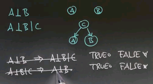
And the answer is that both of them are false. We already saw that conditional independence, as shown over here, doesn't give us absolute independence. So, for example, this is test #1 and test #2. You might or might not have cancer. Our first test gives us information about whether you have cancer or not. As a result, we've changed our prior probability for the second test to come in positive. That means that conditional independence does not imply absolute independence, which means this assumption here falls, and it also turns out that if you have absolute independence, things might not be conditionally independent for reasons that I can't quite explain so far, but that we will learn about next.
Confounding Cause
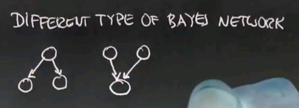
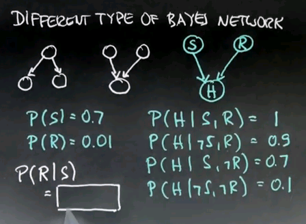
For my next example, I will study a different type of Bayes network. Before, we've seen networks of the following type, where a single hidden cause caused 2 different measurements. I now want to study a network that looks just like the opposite, with 2 independent hidden causes, but they get confounded within a single observational variable.
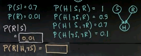
I would like to use the example of happiness. Suppose I can be happy or unhappy. What makes me happy is when the heather is sunny or if I get a raise in my job, which means I make more money. So let's call this sunny (S), let's call this a raise (R), call this happiness (H).
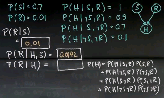
Perhaps the probability of it being sunny is 0.7, probability of a raise is 0.01. And I will tell you that the probability of being happy is governed as follows. The probability of being happy given that both of these things occur -- I got a raise and it is sunny -- is 1. The probability of being happy given that it is not sunny and I still got a raise is 0.9. The probability of being happy given that it's sunny but I didn't get a raise is 0.7. And the probability of being happy given that it is neither sunny nor did I get a raise is 0.1.
This is a perfectly fine specification of a probability distribution where 2 causes affect the variable down here, the happiness (H).
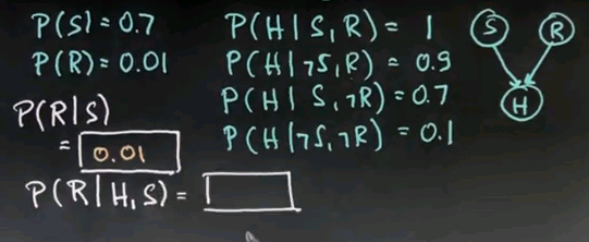
So I'd like you to calculate for me the following questions. The probability of a raise given that it is sunny, according to this model. Please enter your answer over here.
Note: the answer is 0.01 because R and S are absolutely independent.
Explaining Away
Let me talk about a really interesting special instance of Bayes net reasoning which is called explaining away. And I'll first give you the intuitive answer, then I wish you to compute probabilities for me that manifest the explain away effect in a Bayes network of this type.
Explaining away means that if we know that we are happy, then sunny weather can explain away the cause of happiness. If I then also know that it's sunny, it becomes less likely that I received a raise. Let me put this differently. Suppose I'm a happy guy on a specific day and my wife asks me, "Sebastian, why are you so happy? Is it sunny, or did you get a raise?" If she then looks outside and sees it is sunny, then she might explain to herself, "Well, Sebastian is happy because it is sunny. That makes it effectively less likely that he got a raise because I could already explain his happiness by it being sunny." If she looks outside and it is rainy, it makes it more likely I got a raise, because the weather can't really explain my happiness. In other words, if we see a certain effect that could be caused by multiple causes, seeing one of those causes can explain away any other potential cause of this effect over here (H).
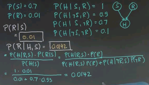
So let me put this in numbers and ask you the challenging question of what's the probability of a raise given that I'm happy and it's sunny?
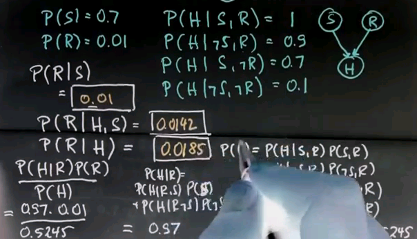
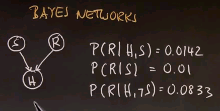
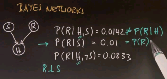
The answer is approximately 0.0142, and it is an exercise in expanding this term (P(R|H,S))using Bayes' rule, using total probability, which I'll just do for you. Using Bayes' rule, you can transform this into P(H|R,S) times P(R|S)/P(H|S) over P(H|S). We observe the conditional independence of R and S to simplify this to just P of R, and the denominator is expanded by folding in R and not R, P(S|R,S)P(R)+P(H|~R,S)P(~R), which is total probability. We can now read off the numbers from the tables over here, which gives us 1 times 0.01 divided by this expression that is the same as the expression over here, so 0.01 plus this thing over here, which you can find over here to be 0.7, times this guy over here, which is 1 minus the value over here, 0.99, which gives us approximately 0.0142.
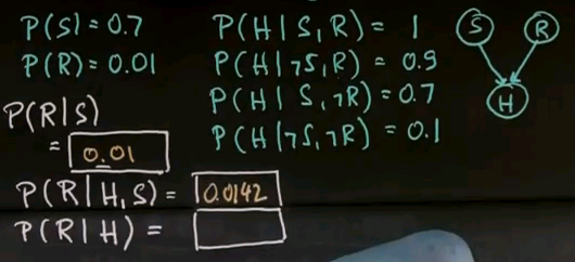
Now, to understand the explain away effect, we have to compare this to the probability of a raise given that we're just happy and we don't know anything about the weather. So let's do that exercise next. So my next quiz is, what's the probability of a raise given that all I know is that I'm happy and I don't know about the weather? This happens once again to be a pretty complicated question, so take your time.
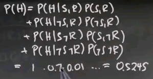
So this is a difficult question. Let me compute an auxiliary variable, which is P of happiness (P(H)). That one is expanded by looking at the different conditions that can make us happy. P(H|S,R) * P(S,R), which is of course the product of those two (P(S) and P(R)) because they are independent, plus P(H|~S,R) * P(~S,R), plus P(H|S,~R) times P(S,~R), plus the last case P(H|~S,~R) times P(~S,~R).
So this just looks at the happiness under all 4 combinations of the variables that could lead to happiness. And you can plug those straight in. This one over here (P(H|S,R)) is 1, and this one over here (P(S,R)) is the product of S and R, which is 0.7 times 0.01. And as you plug all of those in, you get as a result 0.5245. That's P of H (P(H)). Just take some time and do the math by going through these different cases using total probability, and you get this result.
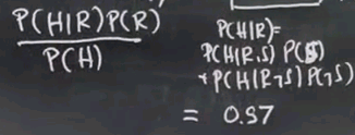
Now armed with this number, the rest now becomes easy, which is we can use Bayes' rule to turn this around. P(H|R) * P(R) / P(H). P(R) we know from over here, the probability of a raise is 0.01. So the only thing we need to compute now is P(H|R). And again, we apply total probability. Let me just do this over here. We can factor P(H|R) as P(H|R,S) * P(S) + P(H|R,~S) * P(~S) and if you plug in the numbers for this, you get 1 times 0.7 plus 0.9 times 0.3. That happens to be 0.97.
So if we now plug this all back into this equation over here, we get 0.97 times 0.01 over 0.5245. This gives us approximately as the correct answer 0.0185.
And if you got this right, I will be deeply impressed about the fact you got this right. But the interesting thing now to observe is if we happen to know it's sunny and I'm happy, then the probability of a raise is 1.4%, 0.014. If I don't know about the weather and I'm happy, then the probability of a raise goes up to about 1.85%. Why is that? Well, it's the explaining away effect. My happiness is well explained by the fact that it's sunny. So if someone observes me to be happy and asks the question, "Is this because Sebastian got a raise at work?" Well, if you know it's sunny and this is a fairly good explanation for Sebastian being happy, and you don't have to assume Sebastian got a raise. If you don't know about the weather, then obviously the chances are higher that the raise caused my happiness, and therefore this number goes up from 0.014 to 0.018.
Let me ask you one final question in this next quiz, which is the probability of the raise given that I look happy and it's not sunny. This is the most extreme case for making a raise likely because I am a happy guy, and it's definitely not caused by the weather. So it could be just random, or it could be caused by the raise. So please calculate this number for me and enter it into this box.
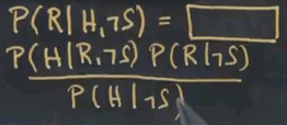
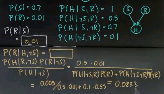
Well, the answer follows the exact same scheme as before, with S being replaced by not S. So this should be an easier question for you to answer. P(R|H,~S) can be inverted by Bayes' rule to be as follows.
Once we apply Bayes' rule, as indicated over here where we swapped H to the left side and R to the right side, you can observe that this value over here (P(R|H,~S)) can be readily found in the table. It's actually the 0.9 over there. This value over here (P(R|~S)), the raise is independent of the weather by virtue of our Bayes network, so it's just 0.01. And as before, apply total probability to the expression over here (P(H|~S)), and we obtain off this quotient over here that these 2 expressions are the same. P(H|~S,~R) is the value over here, and the 0.99 is the complement of probability of R taken from over here and that ends up to be 0.0833.
Conditional Dependence
It's really interesting to compare this to the situation over here. In both cases I'm happy, as shown over here, and I ask the same question, which is whether I got a raise at work, as R over here. But in one case I observe that the weather is sunny; in the other one it isn't. And look what it does to my probability of having received a raise. The sunniness perfectly well explains my happiness, and my probability of having received a raise ends up to be a mere 1.4%, or 0.014. However, if my wife observes it to be non-sunny, then it is much more likely that the cause of my happiness is related to a raise at work, and now the probability is 8.3%, which is significantly higher than the 1.4% before.
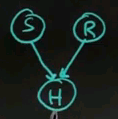
Now this is a Bayes network of which S and R are independent, but H adds a dependence between S and R.
Let me talk about this in a little bit more detail on the next paper.
So here's our Bayes network again:
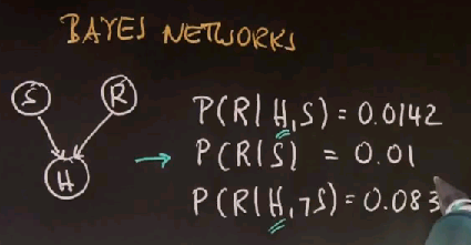
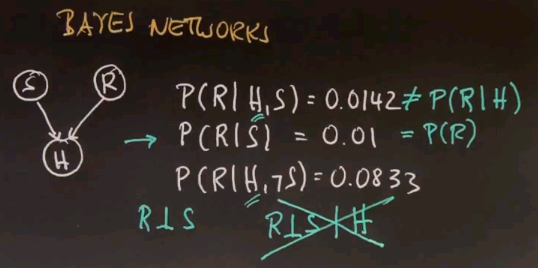
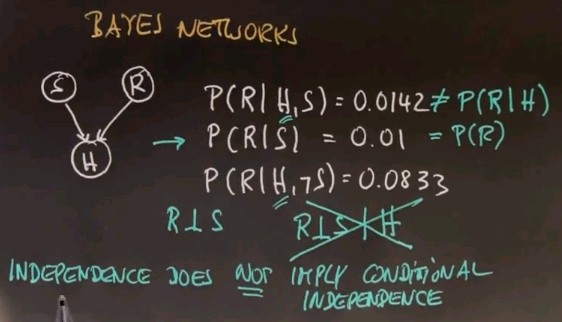
In our previous exercises, we computed for this network that the probability of a raise of R given any of these variables shown here was as follows.
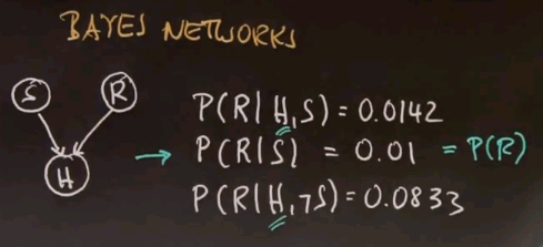
The really interesting thing is that in the absence of information about H, which is the middle case over here,
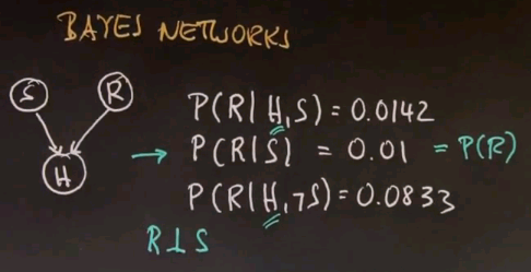
the probability of R is unaffected by knowledge of S -- that is, R and S are independent. This is the same as probability of R,
and R and S are independent.
However, if I know something about the variable H, then S and R become dependent -- that is, knowing about my happiness over here renders S and R dependent. This is not the same as probability of just R given H.
Obviously it isn't because if I now vary S from S to not S, it affects my probability for the variable R. That is a really unusual situation where we have R and S are independent but given the variable H, R and S are not independent any more.
So knowledge of H makes 2 variables that previously were independent non-independent. Or put differently, 2 variables that are independent may not be, in certain cases, conditionally independent. Independence does not imply conditional independence.
General Bayes Net
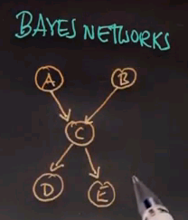
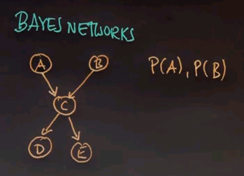
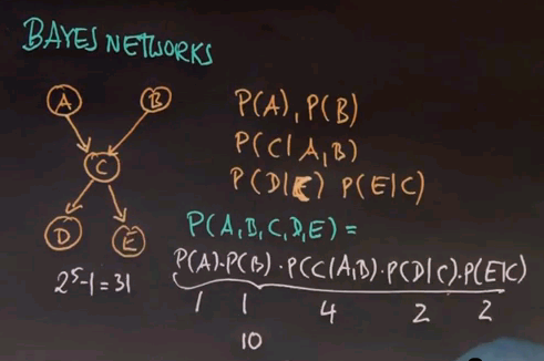
So we're now ready to define Bayes networks in a more general way. Bayes networks define probability distributions over graphs of random variables. Here is an example graph of 5 variables:
and this Bayes network defines the distribution over those 5 random variables. Instead of enumerating all possibilities of combinations of these 5 random variables, the Bayes network is defined by probability distributions that are inherent to each individual node. For node A and B, we just have a distribution of P(A) and P(B) because A and B have no incoming arcs.
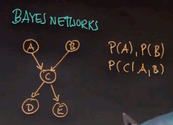
C is a conditional distribution conditioned on A and B:
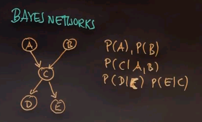
And D and E are conditioned on C:
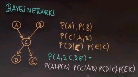
The joint probability represented by a Bayes network is the product of various Bayes network probabilities that are defined over individual nodes where each nodes probability is only conditioned on the incoming arcs. So A has no incoming arc; therefore, we just want is P(A). C has 2 incoming arcs, so we define the probability of C conditioned on A and B. And D and E have 1 incoming arc that's shown over here.
The definition of this joint distribution by using the following factors has one really big advantage. Whereas the joint distribution over any 5 variables requires 25-1, which is 31 probability values, the Bayes network over here only requires 10 such values. P(A) is one value, for which we can derive P(~A). Same for P(B). P(C|A,B) is derived by a distribution over C conditioned on any combination of A and B, of which there are 4 of A and B as binary. P(D|C) is 2 parameters for P(D|C) and P(D|~C). And the same is true for P(E|C). So if you add those up, you get 10 parameters in total.
So the compactness of the Bayes network leads to a representation that scales significantly better to large networks that the combinatorial approach which goes through all combinations of variable values. That is a key advantage of Bayes networks, and that is the reason why Bayes networks are being used so extensively for all kinds of problems.
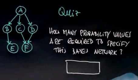
So here is a quiz. How many probability values are required to specify this Bayes network? Please put your answer in the following box.
And the answer is 13. 1 for A, 2 for B, 2 for C, 2 for D, 2 for E and 4 for F.
Simply speaking, any variable that has K inputs requires 2 to the K such variables.
So in total we have 13.
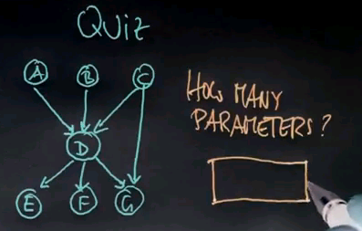
Here's another quiz. How many parameters do we need to specify the joint distribution for this Bayes network over here where A, B and C point into D; D points into E, F and G; and C also points into G? Please write your answer into this box.
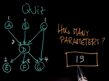
And the answer is 19. 1 for A; 1 for B; 1 for C; 2 for E; 2 for F; 2 arcs point into G, which makes 4; and 3 arcs point into D, 23 is 8. So we get 1, 2, 3, 8, 2, 2, 4. If you add those up it's 19.
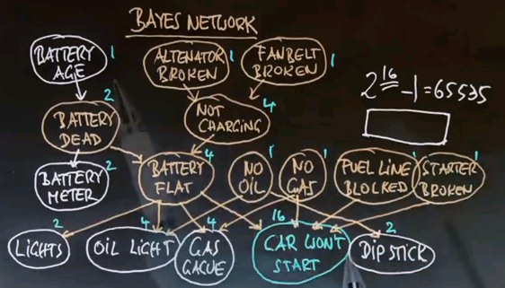
And here is our car network which we discussed at the very beginning of this unit. How many parameters do we need to specify this network? Remember, there are 16 total variables, and the naive joint over the 16 will be 216-1, which is 65,535. Please write your answer into this box over here.
To answer this question, let us add up these numbers. If we add up all these numbers we get 47.
Value of a Network
So it takes 47 numerical probabilities to specify the joint compared to 65,000 if you didn't have the graph-like structure. I think this example really illustrates the advantage of complex Bayes network representations over unstructured joint representations.
D-separation
The next concept I'd like to teach you is called D-separation. And let me start the discussion of this concept by a quiz.
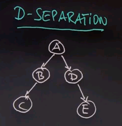
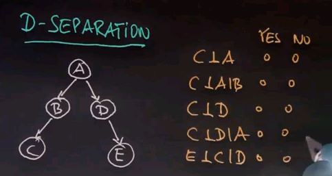
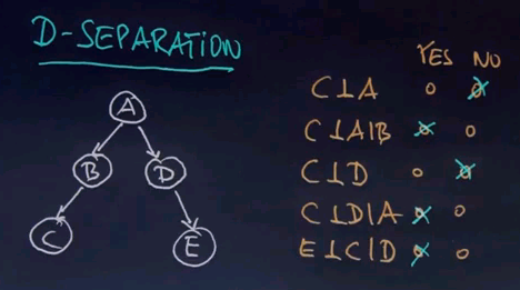
We have here a Bayes network, and I'm going to ask you a conditional independence question. Is C independent of A? Please say yes or no. Is C independent of A given B? Is C independent of D? Is C independent of D given A? And is E independent of C given D?
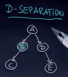
So C is not independent of A. In fact, A influences C by virtue of B. But if you know B, then A becomes independent of C, which means the only determinate into C is B. If you know B for sure, then knowledge of A won't really tell you anything about C. C is also not independent of D, just the same way C is not independent of A. If I learn something about D, I can infer more about C. But if I do know A, then it's hard to imagine how knowledge of D would help me with C because I can't learn anything more about A than knowing A already. Therefore, given A, C and D are independent. The same is true for E and C. If we know D, then E and C become independent.
In this specific example, the rule that we could apply is very, very simple. Any two variables are independent if they're not linked by just unknown variables. So for example, if we know B, then everything downstream of B becomes independent of anything upstream of B. E is now independent of C, conditioned on B. However, knowledge of B does not render A and E independent.
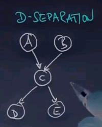
In this graph over here:
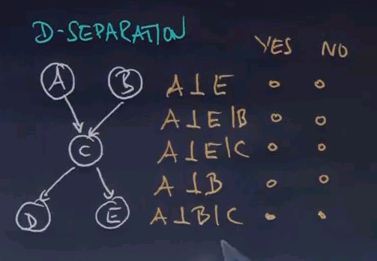
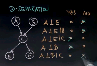
A and B connect to C and C connects to D and E. So let me ask you, is A independent of E, A independent of E given B, A independent of E given C, A independent of B, and A independent of B given C?
And the answer for this one is really interesting. A is clearly not independent of E because through C we can see an influence of A to E. Given B, that doesn't change. A still influences C, despite the fact we know B. However, if we know C, the influence is cut off. There's no way A can influence E if we know C. A is clearly independent of B. They are different entry variables. They have no incoming arcs. But here is the caveat. Given C, A and B become dependent.
So whereas initially A and B were independent, if you give C, they become dependent. And the reason why they become dependent we've studied before. This is the explain away effect. If you know, for example, C to be true, then knowledge of A will substantially affect what we believe about B. If there's 2 joint causes for C and we happen to know A is true, we will discredit cause B. If we happen to know A is false, we will increase our belief for the cause B. That was an effect we studied extensively in the happiness example I gave you before. The interesting thing here is we are facing a situation where knowledge of variable C renders previously independent variables dependent.
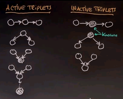
This leads me to the general study of conditional independence in Bayes networks, often called D-separation of reachability. D-separation is best studied by so-called active triplets and inactive triplets where active triplets render variables dependent and inactive triplets render them independent. Any chain of three variables like this makes the initial and final variable dependent if all variables are unknown. However, if the centre variable is known -- that is, it's behind the conditioning bar -- then this variable and this variable become independent. So if we have a structure like this and it's "cut off" by a known variable in the middle, that separates or de-separates the left variable from the right variable, and they become independent. Similarly, any structure like this renders the left variable and the right variable dependent unless the centre variable is known, in which case the left and right variable become independent. Another active triplet now requires knowledge of a variable. This is the explain away case. If this variable is known for a Bayes network that converges into a single variable, then this variable and this variable over here become dependent. Contrast this with a case where all variables are unknown. A situation like this means that this variable on the left or on the right are actually independent. In a single final example, we also get dependence if we have the following situation: a direct successor of a conversion variable is known. So it is sufficient if a successor of this variable is known. The variable itself does not have to be known, and the reason is if you know this guy over here, we get knowledge about this guy over here. And by virtue of that, the case over here essentially applies.
If you look at those rules, those rules allow you to determine for any Bayes network whether variables are dependent or not dependent given the evidence you have. If you colour the nodes dark for which you do have evidence, then you can use these rules to understand whether any 2 variables are conditionally independent or not.
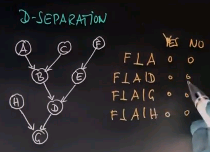
So let me ask you for this relatively complicated Bayes network the following questions. Is F independent of A? Is F independent of A given D? Is F independent of A given G? And is F independent of A given H? Please mark your answers as you see fit.
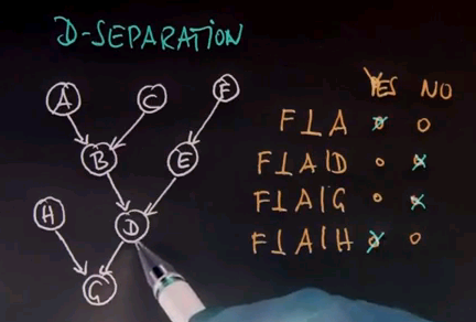
And the answer is yes, F is independent of A. What we find for our rules of D-separation is that F is dependent on D and A is dependent on D. But if you don't know D, you can't govern any dependence between A and F at all. If you do know D, then F and A become dependent. And the reason is B and E are dependent given D, and we can transform this back into dependence of A and F because B and A are dependent and E and F are dependent. There is an active path between A and F which goes across here and here because D is known. If we know G, the same thing is true because G gives us knowledge about D, and D can be applied back to this path over here. However, if you know H, that's not the case. So H might tell us something about G, but it doesn't tell us anything about D, and therefore, we have no reason to close the path between A and F. The path between A and F is still passive, even though we have knowledge of H.
Congratulations
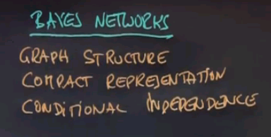
So congratulations. You learned a lot about Bayes networks. You learned about the graph structure of Bayes networks, you understood how this is a compact representation, you learned about conditional independence, and we talked a little bit about applications of Bayes networks to interesting reasoning problems.
But by all means this was a mostly theoretical unit of this class, and in future classes we will talk more about applications. The instrument of Bayes networks is really essential to a number of problems. It really characterizes the sparse dependence that exists in many real problems like in robotics and computer vision and filtering and diagnostics and so on. I really hope you enjoyed this class, and I really hope you understood in depth how Bayes networks work.
