AI class unit 6
These are my notes for unit 6 of the AI class.
Unsupervised Learning
Unsupervised Learning
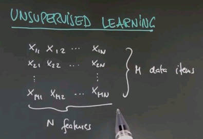
So welcome to the class on unsupervised learning. We talked a lot about supervised learning in which we are given data and target labels. In unsupervised learning we're just given data. So here is a data matrix of data items of n features each. There's m in total.
So the task of unsupervised learning is to find structure in data of this type. To illustrate why this is an interesting problem let me start with a quiz. Suppose we have two feature values. One over here, and one over here, and our data looks as follows. Even though we haven't been told anything in unsupervised learning, I'd like to quiz your intuition on the following two questions: First, is there structure? Or put differently do you think there's something to be learned about data like this, or is it entirely random? And second, to narrow this down, it feels that there are clusters of data the way I do it. So how many clusters can you see? And I give you a could of choices, 1, 2, 3, 4, or none.
The answer to the first question is yes, there is structure. Obviously these data seem not to be completely randomly determinate. There seem to be, for me, two clusters. So the correct answer for the second question is 2. There's a cluster over here, and there's a cluster over here. So one of the tasks of unsupervised learning will be to recover the number of clusters, and the centre of these clusters, and the variance of these clusters in data of the type I've just shown you.
Question
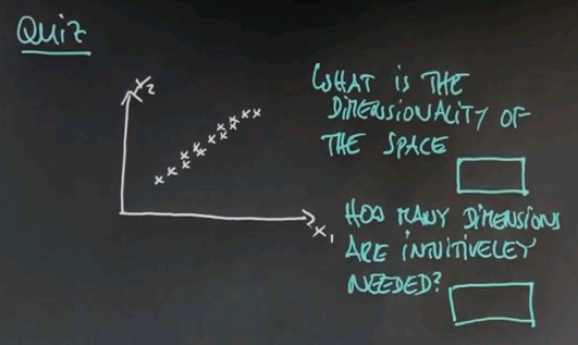
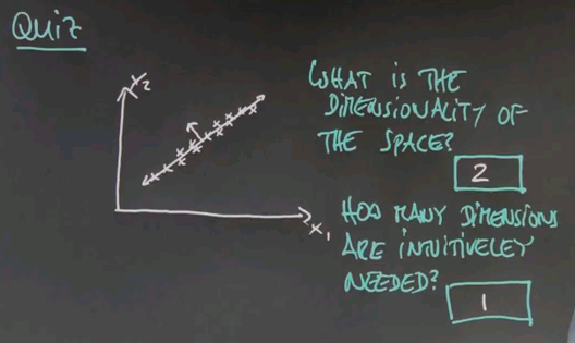
Let me ask you a second quiz. Again, we haven't talked about any details. But I would like to get your intuition on the following question. Suppose in a two-dimensional space all the data lies as follows. This may be reminiscent of the question I asked you for housing prices and square footage. Suppose we have two axes, x1 and x2. I'm going to ask you two questions here. One is what is the dimensionality of this space in which this data falls, and the second one is an intuitive question which is how many dimensions do you need to represent this data to capture the essence. And again, this is not a clear crisp 0 or 1 type question, but give me your best guess. How many dimensions are intuitively needed?
And here are the answers that I would give to these two questions. Obviously the dimensionality of the data is two, there's an x dimension and a y dimension. But I believe you can represent this all in one dimension. If you pick this dimension over here then the major variation of the data goes along this dimension. If you were for example to look at the orthogonal dimension, in this direction over here, you would find that there's very little variation in the second dimension, so if you only graphed your data along one dimension you'd be doing well.
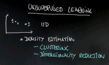
Now this is an example of unsupervised learning where you find structure in terms of lower dimensionality of data. And especially for very high dimensional data, like image data, this is an important technique. So I talk a little bit later in this unit about dimensionality reduction. So in this class we learn about clustering, dimensionality reduction, and we'll apply it to a number of interesting problems.
Terminology
So to start with some lingo about unsupervised learning. If you look at this as a probabilist, you're given data, and we typically assume the data is IID, which means identically distributed and independently drawn from the same distribution. So a good chunk of unsupervised learning seeks to recover the underlying -- the density of the probability distribution that generated the data. It's called density estimation. As we find out our methods for clustering are versions of density estimation using what's called mixture models. Dimensionality reduction is also a method for doing density estimation. And there are many others.
Unsupervised learning can be applied to find structure in data. One of the fascinating ones that I believe exists is called blind signals separation. Suppose you are given a microphone, and two people simultaneously talk, and you record the joint of both of those speakers. Blind source separation or blind signal separation addresses the question of can you recover those two speakers and filter the data into two separate streams, one for each speaker. Now this is a really complicated unsupervised learning task, but is one of the many things that don't require target signals as unsupervised learning yet make for really interesting learning problems. This can be construed as an example of what's called factor analysis where each speaker is a factor in the joint signal that your microphone records. There are many other examples of unsupervised learning. I will show you a few in a second.
Google Street View and Clustering
Here is one of my favourite examples of unsupervised learning -- one that is yet unsolved. At Google, I had the opportunity to participate in the building of Street View, which is a huge photographic database of many many streets in the world. As you dive into Street View you can get ground imagery of almost any location in the world -- like this house here that I chose at random. In these images there is vast regularities. You can go somewhere else and you'll find that the type of objects visible in Street View is not entirely random. For example, there is many images of homes, many images of cars, trees, pavement, lane markers, stop signs, just to name a few. So one of the fascinating unsolved unsupervised learning tasks is: can you take hundreds of billions of images as comprised in the Street View data set and discover from it that there are concepts such as trees, lane markers, stop signs, cars and pedestrians? It seems to be tedious to hand label each image for the occurrence of such objects. And attempts to do so has resulted in very small image data sets. Humans can learn from data even without explicit target labels. We often just observe. In observing we apply unsupervised learning techniques. So one of the great, great open questions of artificial intelligence is: can you observe many intersections and many streets and many roads and learn from it what concepts are contained in the imagery?
Of course I can't teach you anything as complex in this class. I don't even know the answer myself. So let me start with something simple. Clustering. Clustering is the most basic form of unsupervised learning. And I will tell you about two algorithms that are very related. One is called k-means, and one is called expectation maximisation. K-means is a nice, intuitive algorithm to derive clusterings. Expectation maximisation is a probabilistic generalisation of k-means. They will be derived from first principles.
k-Means Clustering Example
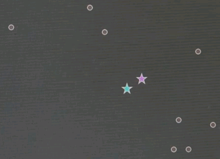
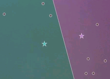
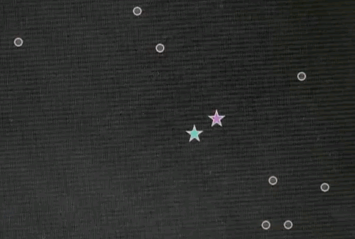
Let me explain k-means by an example. Suppose we're given the following data points in a two-dimensional space. K-means estimates for a fixed number of k, here k=2. The best centres of clusters representing those data points. Those are found iteratively by the following algorithm.
Step 1: Guess cluster centres at random, as shown over here with the two stars.
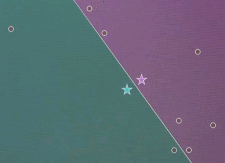
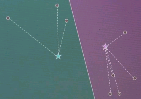
Step 2: Assign to each cluster centre, even though they are randomly chosen, the most likely corresponding data points. This is done by minimising Euclidean distance. In particular, each cluster centre represents half of the space. And the line that separates the space between the left and right cluster centre is the equidistant line, often called a Voronoi graph.
All the data points on the left correspond to the red (green) cluster, and the ones on the right to the green (purple) cluster.
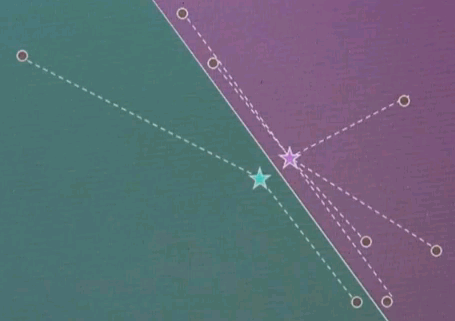
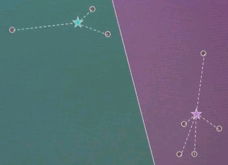
Step 3: Given now we have a correspondence between the data points and the cluster centres, find the optimal cluster centre that corresponds to the points associated with the cluster centre. Our red (green) cluster centre has only two data points attached. So the optimal cluster centre would be the halfway point in the middle.
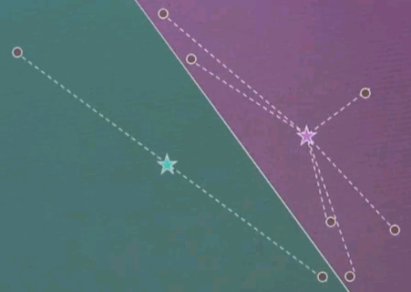
Our right cluster centre has more than two data points attached, yet it isn't placed optimally, as you can see as they move with the animation back and forth. By minimising the joint quadratic distance to all of those points the new cluster centre is attained at the centre of those data points.
Now the final step is iterate. Go back and reassign cluster centres.
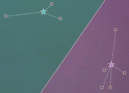
Now the Voronoi diagram has shifted, and the points are associated differently, and then re-evaluate what the optimal cluster centre looks like given the associated points.
And in both cases we see significant motion. Repeat.
Now this is the clustering. The point association doesn't change, and as a result, we just converged.
k-Means Algorithm
Note: For nearest distance, you may assume Euclidean. However, you can also generally substitute other distance metrics.
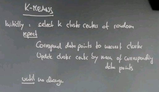
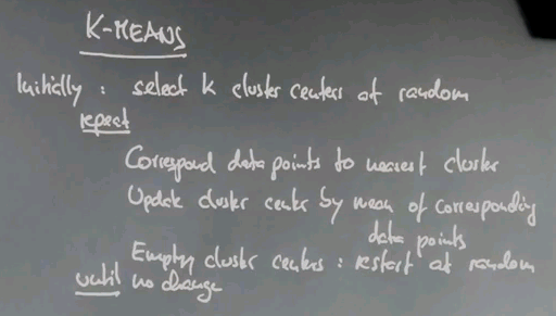
You just learned about an exciting clustering algorithm that's really easy to implement called k-means. To give you the algorithm in pseudocode initially we select k cluster centres at random and then we repeat. In a correspondence step, we correspond all the data points to the nearest cluster centre, and then we calculate the new cluster centre by the mean of the corresponding data points. We repeat this until nothing changes any more.
Now special care has to be taken if a cluster centre becomes empty -- that means no data point is associated. In which case we just restart cluster centres at random that have no corresponding points. Empty cluster centres restart at random.
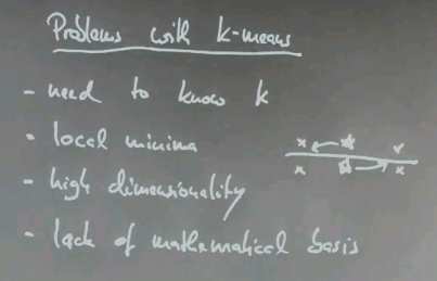
This algorithm is known to converge to a locally optimal clustering of data points. The general clustering problem is known to be NP-hard. So a locally optimal solution, in a way, is the best we can hope for. Now let me talk about problems with k-means. First we need to know k, the number of cluster centres. As I mentioned, the local minima. For example, for four data points like this and two cluster centres that happen to be just over here, with the separation line like this, there would be no motion of k-means, even though moving one over here and one over there would give a better solution.
There's a general problem of high dimensionality of the space that is not dissimilar from the way k-nearest neighbour suffers from high dimensionality. And then there's lack of mathematical basis. Now if you're a practitioner, you might not care about a mathematical basis, but for the sake of this class, let's just care about it.
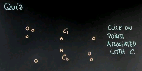
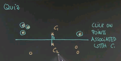
So here's a first quiz for k-means. Given the following two cluster centres, c1 and c2, click on exactly those points that are associated with c1 and not with c2.
And the answer is these four points over here. The reason is, if you draw the line of equal distance between c1 and c2, the separation of these two cluster areas falls over here. c2 is down there, c1 is up here.
Question
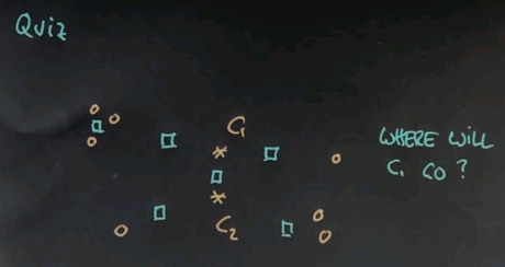
So here's my second quiz. Given the association we just derived for c1, where do you think the new cluster centre, c1, will be found after a single step of estimating its best location given the associated points? I'll give you a couple of choices. Please click on the one that you find the most plausible.
And the answer is over here. These four data points are associated with c1, so we can safely ignore all the other ones. This one over here would be at the centre of the three data points over here, but this one pulls back this data point drastically towards it. This is about the best trade-off between these three points over here that all have a string attached and pull in this direction, compared to this point over here. Any of the other ones don't even lie between those points and therefore won't be good cluster centres. The one over here is way too far to the right.
Question
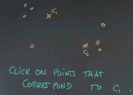
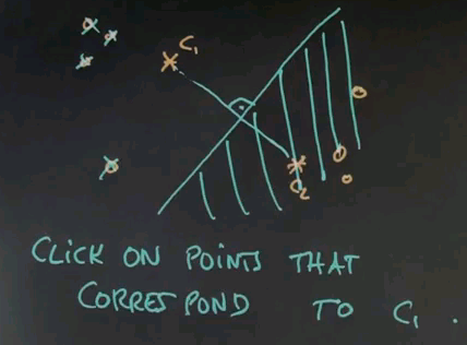
In our next quiz let's assume we've done one iteration and the cluster centre of c1 moved over there and c2 moved over here. Can you once again click on all those data points that correspond to c1?
And the answer is now simple. It's this one over here. This one, this one, and this one. And the reason is, the line separating both clusters runs around here. That means all the area over here is c2 territory, and the area over here is c1 territory.
Obviously as we now iterate k-means, these clusters that have been moved straight over here will be able to stay, whereas, c2 will end up somewhere over here.
Expectation Maximisation
So, let's now generalise k-means into expectation maximisation.
Expectation maximisation is an algorithm that uses actual probability distributions to describe what we're doing, and it's in many ways more general, and it's also nice in that it really has a probabilistic basis.
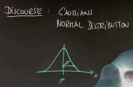
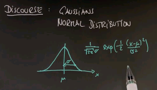
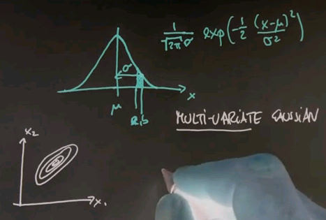
To get there, I have to take the discourse and tell you all about Gaussians, or the normal distribution, and the reason is so far we've just encountered discrete distributions, and Guassians will be the first example of a continuous distribution. Many of you know that a Gaussian is described by an identity that looks as follows, where the mean is called mu, and the variance is called sigma or sigma squared.
And for any x along the horizontal axis, the density is given by the following function: 1 over square root of 2 pi times sigma, and then an exponential function of minus a half of x minus mu squared over sigma squared.
This function might look complex, but it's also very, very beautiful. It peaks at x equals mu, where the value in the exponent becomes zero, and towards plus or minus infinity it goes to zero quickly. In fact, exponentially fast. The argument inside is a quadratic function. The exponential function makes it exponential. And this over here is a normaliser to make sure that the area underneath sums up to one, which is a characteristic of any probability density function.
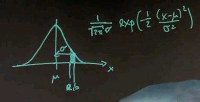
If you map this back to our discrete random variables, for each possible x, we can now assign a density value, which is the function of this, and that's effectively the probability that this x might be drawn. Now the space itself is infinite, so any individual value will have a probability of zero, but what you can do is you can make an interval, A and B, and the area underneath this function is the total probability that an experiment will come up between A and B. Clearly it's more likely to generate values around mu than it is to generate values in the periphery somewhere over here.
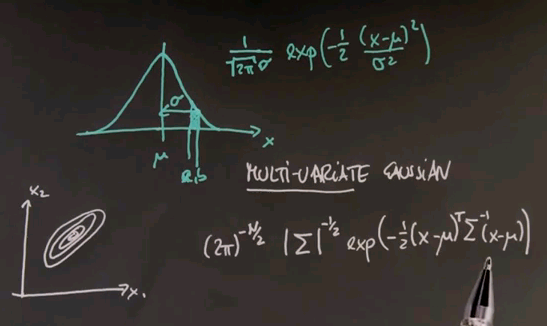
And just for completeness, I'm going to give you the formula for what's called the multivariate Gaussian, where multivariate means nothing else but we have more than one input variable. You might have a Gaussian over a two-dimensional space or a three-dimensional space. Often these Gaussians are drawn by what's called level sets, sets of equal probability. Here's one in a two-dimensional space, x1 and x2.
The Gaussian itself can be thought of as coming out of the paper towards me, where the most likely or highest point of probability is the centre over here. And these rings measure areas of equal probability.
The formula for a multivariate Gaussian looks as follows. N is the number of dimensions in the input space. Sigma is a covariance matrix that generalises the value over here. And the inner product inside the exponential is now done using linear algebra where this is the difference between a probe point and the mean vector mu transposed sigma to the minus 1 times x minus mu.
You can find this formula in any textbook or web page on Gaussians or multivariate normal distributions. It looks cryptic at first, but the key thing to remember is that it's just a generalisation of the one-dimensional case. We have a quadratic area over here as manifested by the product of this guy and this guy. We have a normalisation by a variance or covariance as shown by this number over here or the inverse matrix over here. And then this entire thing is an exponential form in both cases, and the normaliser looks a little more different in the multivariate case, but all it does is make sure that the volume underneath adds up to 1 to make it a legitimate probability density function.
For most of this explanation, I will stick with one-dimensional Gaussians, so all you have to do is to worry about this formula over here, but this is given just for completeness.
Gaussian Learning
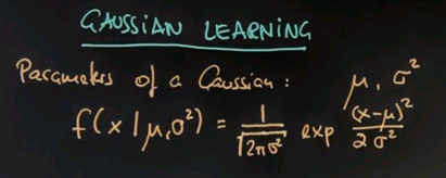
Note: The formula is missing a minus sign: f ( x,mu,sigma^2 ) = 1 / ( sqrt (2 * pi * sigma^2) * exp ( -(x-mu)^2 / ( 2 * sigma^2 )
I will now talk about fitting Gaussians to data or Gaussian learning. You may be given some data points, and you might worry about what is the best Gaussian fitting the data? Now, to explain this, let me first tell you what parameters characterises a Gaussian. In the one-dimensional case, it is mu and sigma squared. Mu is the mean, sigma squared is called the variance. So if we look at the formula of a Gaussian, it's a function over any possible input x, and it requires knowledge of mu and sigma squared. And as before, I'm just restating what I said before, we get this function over here that specifies any probability for a value x given specific mu and sigma squared.
So suppose we wish to fit data, and our data is one-dimensional, and it looks as follows.
Just looking at this diagram makes me believe that there's a high density of data points over here and a fading density of data points over there, so maybe the most likely Gaussian will look a little bit like this where this is mu and this is sigma.
There are really easy formulas for fitting data to Gaussians, and I'll give you the result right now. The optimal or most likely mean is just the average of the data points. So there's M data points, x<sub1 to xM. The average will look like this. The sum of all data points divided by the total number of data points.
That's called the average. And once you calculate the average, the sigma squared is obtained by a similar normalisation in a slightly more complex sum.
We sum the deviation from the mean and compute the average deviation to the square from the mean, and that gives us sigma squared. So, intuitively speaking, the formulas are really easy. Mu is the mean, or the average. Sigma squared is the average quadratic deviation from the mean, as shown over here.
Maximum Likelihood
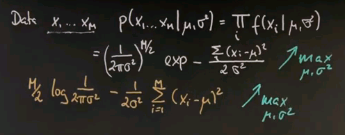
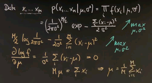
Now I want to take a second to convince ourselves this is indeed the maximum likelihood estimate of the mean and the variance. Suppose our data looks like this -- there's M data points. And the probability of those data points for any Gaussian model -- mu and sigma squared is the product of any individual data likelihood xi. And if you plug in our Gaussian formula, you get the following.
This is the normaliser multiplied M times where the square root is now drawn into the half over here. And here is our joint exponential, where we took the product of the individual exponentials and moved it up straight in here where it becomes a sum. So the best estimates for mu and sigma squared are those that maximise this entire expression over here for a given data set x1 to xm.
So we seek to maximise this over the unknown parameters mu and sigma squared. And now I will apply a trick. Instead of maximising this expression, I will maximise the logarithm of this expression. The logarithm is a monotonic function. So let's maximise instead the logarithm where this expression over here resolves to this expression over here. The multiplication becomes a minus sign from over here, and this is the argument inside the exponent written slightly differently but pulling the 2 sigma squared to the left.
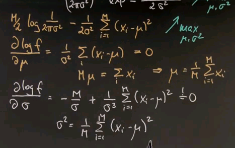
So let's maximise this one instead. The maximum was obtained where the first derivative is zero. If we do this for our variable mu, we take the log f expression and compute the derivative with respect to mu, we get the following. This expression does not depend on mu at all, so it falls out. And we instead get this expression over here, which we've set to zero. And now we can multiply everything by sigma squared, it's still zero, and then bring the xi to the right and the mu to the left. The sum over all E of the mu is mu equals sum over i, xi.
Hence, we proved that the mean is indeed the maximum likelihood estimate for the Gaussian. This is now easily repeated for the variance. If you compute the derivative of this expression over here with respect to the variance, we get minus M over sigma, which happens to be the derivative of this expression over here. Keep in mind that the derivative of a logarithm is just its internal argument times by chain rule -- the derivative of the internal argument. Which if you work it out becomes this expression over here. And this guy over here changes signs but becomes the following. And again, you move this guy to the left side, multiply by sigma cubed, and divide by m. So we get the following result over here.
You might take a moment to verify these steps over here. I was a little bit fast, but this is relatively straight forward mathematics. And if you verify them you will find that the maximum likelihood estimate for sigma squared is the average deviation of data points from the mean mu. This gives us a very nice basis to fit Gaussians to data points.
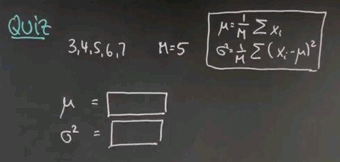
So keeping these formulas in mind, here's a quick quiz, in which I ask you to actually calculate the mean and variance for a data sequence. So suppose the data you observe is 3, 4, 5, 6, and 7. There is 5 data points. Compute for me the mean and the variance using the maximum likelihood estimator I just gave you.
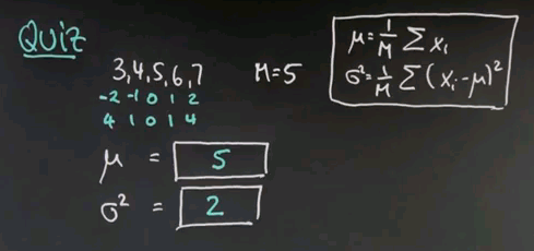
So the mean is obviously 5, it's the middle value over here. If I add those things together I get 25 and divide by 5. The average value over here is 5. The more interesting case is sigma squared, and I do this in the following steps. I subtract 5 from each of the data points for which I get -2, -1, 0, 1, and 2. I square those differences, which gives me 4, 1, 0, 1, 4. And now I compute the mean of those square differences. To do so I add them all up, which is 10. 10 divided by 5 is 2, and sigma squared equals 2.
Question
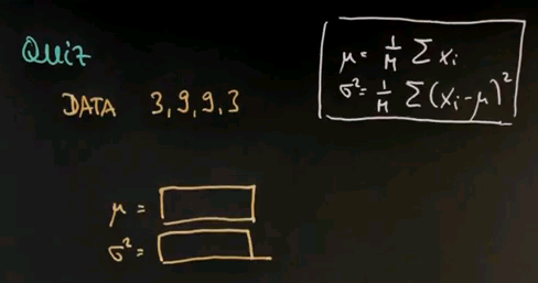
Here's another quiz. Suppose my data looks as follows -- 3, 9, 9, 3. Compute for me mu and sigma squared using the maximum likelihood estimator I just gave you.
And the answer is relatively easy. 3 + 9 + 9 + 3 = 24. Divided by m = 4 is 6. So the mean value is 6. Subtracting the mean from the data gives us -3, 3, 3, and -3. Squaring those gives us 9, 9, 9, 9 and the mean of four 9s equals 9.
Question
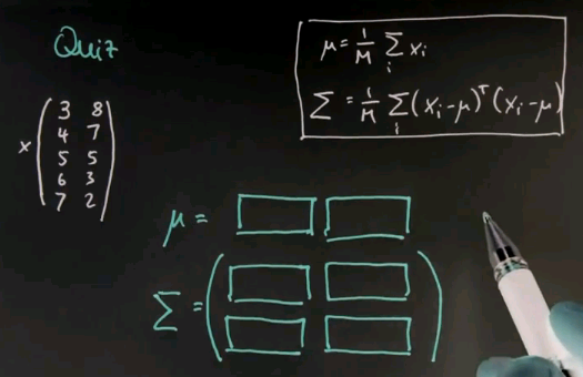
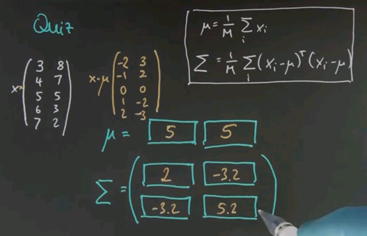
I now have a more challenging quiz for you in which I give you multivariate data, in this case two-dimensional data. So suppose my data goes as follows. In the first column I get 3, 4, 5, 6, 7. These are five data points and this is the first feature. And the second feature will be 8, 7, 5, 3, 2. The formulas for calculating mu and the covariance matrix sigma generalise the ones we studied before and they are given over here. So what I would like you to compute is the vector mu, which now has two values, on for the first and one for the second column and the variance sigma, which now has four different values, using the formula shown over here.
Now the mean is calculated as before independently for each of the two features here. 3, 4, 5, 6, 7; the mean is 5. 8, 7, 5, 3, 2; the mean is 5 again. Easy calculation. If you subtract the mean from the data we get the following matrix, and now we just have to plug it in. For the main diagonal elements you get the same formula as before. You can do this separately for each of the two columns. But for the off-diagonal elements you just have to plug it in. So this is the result after plugging it in and you might just want to verify it using a computer.
Gaussian Summary
So this finishes the lecture on Gaussians. You learned about what a Gaussian is. We talked about how to fit them from data, and we even talked about multivariate Gaussians. But even though I asked you to fit one of those the ones we're going to focus on right now is the one-dimensional Gaussian. So let's now move back to the expectation maximisation algorithm.
EM as Generalization of k-Means
It is now really easy to explain expectation maximisation as a generalisation of k-means. Again we have a couple of data points here and two randomly chosen cluster centres.
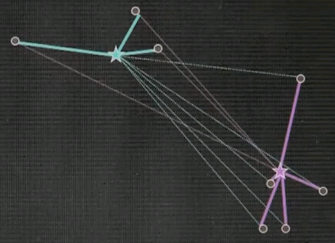
But in the correspondence step instead of making a hard correspondence we make a soft correspondence.
Each data point is attracted to a cluster centre in proportion to the posterior likelihood which we will define in a minute. In the adjustment step, or the maximisation step, the cluster centres are being optimised just like before but now the correspondence is a soft variable and they correspond to all data points in different strengths not just the nearest ones.
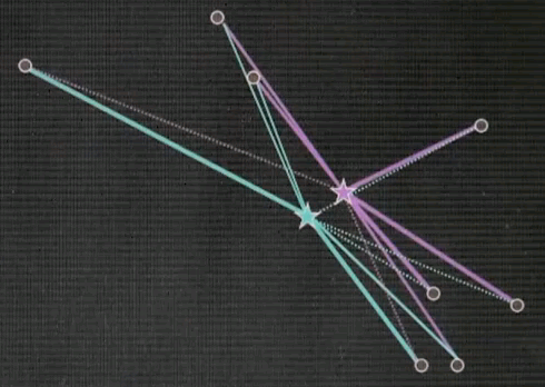
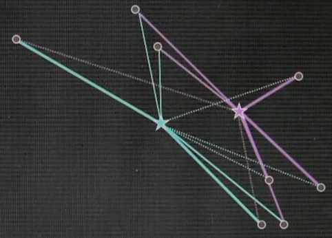
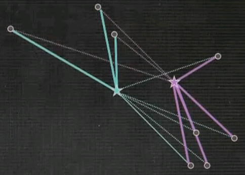
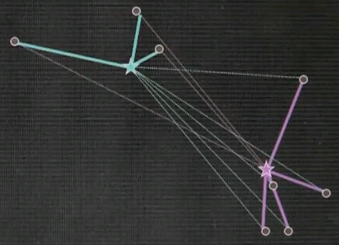
As a result, in EM the cluster centres tend not to move as far as in k-means. They move in a smoother way.
A new correspondence over here gives us different strength as indicated by the different colouring of the links and another relaxation step gives us better cluster centres.
And as you can see, over time,
gradually the EM will then converge to about the same solution as k-means. However, all the correspondences are still alive. Which means there is not a 0, 1 correspondence, there is a soft correspondence which relates to a posterior probability, which I will explain next.
EM Algorithm
The model of expectation maximisation is that each data point is generated from what's called a mixture. The sum over all possible classes, or clusters, of which there are K, we draw a class at random with a prior probability of p of the class C=i and then we draw the data point x from the distribution correspondent with its class over here. The way to think about this, if there is K different cluster centres shown over here each one of those has a generic Gaussian attached.
In the generative version of expectation maximisation you first draw a cluster centre and then we draw from the Gaussian attached to this cluster centre.
The unknowns here are the prior probabilities for each cluster centre which we will call pii and the mui and in the general case sigmai for each of the individual Gaussian. Where i = 1 all the way to K.
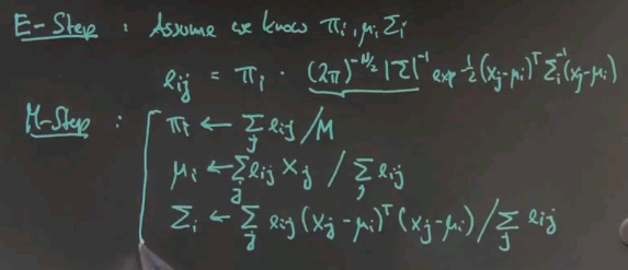
Expectation maximisation iterates 2 steps just like k-means. One is called the E step, or expectation step for which we assume that we know the Gaussian parameters and the pii. With those known values calculating the sum over here is a fairly trivial exercise. This is our known formula for a Gaussian we just plug that it and this is a fixed probability. Sum over all possible classes.
So you get for eij the probability that the j-th data point corresponds to cluster centre number i pii times the normaliser times the Gaussian expression. Where we have a quadratic of xj minus mui times sigmai to the minus one times the same thing again over here.
These are the probabilities that the j-th data point corresponds to the i-th cluster centre under the assumption that we do know the parameters pii, mui and sigmai.
In the M-step we now figure out where these parameters should have been. For the prior probability of each cluster centre we just take the sum over all the eij's, over all data points divided by the total number of data points. The mean is obtained by the weighted mean of the xj's normalised by the sum of eij's and finally the sigma is obtained as a sum over the weighted expression like this and this is the same expression as before and now again we are normalising over the sum over all eij's.
And these are exactly the same calculations as before when we fit a Gaussian but just weighted by the soft correspondence of a data point to each Gaussian. And this weighting is relatively straightforward to apply in Gaussian fitting.
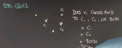
Let's do a very quick quiz for EM. Suppose we're given three data points and two cluster centres. And the question is, does this point over here called x1 correspond to ci or c2 or both of them? Please check exactly one of these three different check boxes here.
And the answer is both of them. And the reason is x1 might be closer to c2 than c1, but the correspondence in EM is soft, which means each data point always corresponds to all cluster centres. It is just that this correspondence over here is much stronger than the correspondence over here.
Question
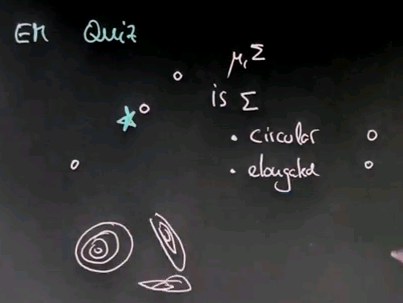
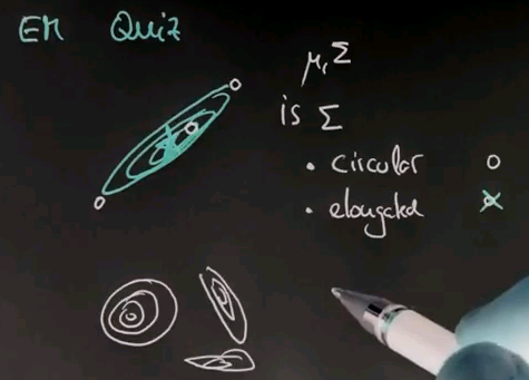
Here's another EM quiz. For this quiz we will assume the degenerative case of three data points and just one cluster centre. My question pertains to the shape of the Gaussian after fitting. Specifically mu and sigma. And the question is, is sigma circular, which would be like this, or elongated, which would be like this or like this?
And the answer is, of course, elongated. As you look over here, what you find is that this is the best Gaussian describing the data points, and this is what EM will calculate.
Question
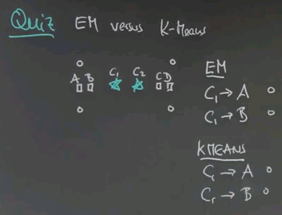
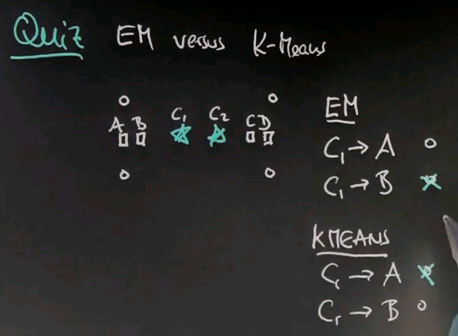
This is a quiz in which I compare EM versus k-means. Suppose we are given four data points, as indicated by those circles. Suppose we have two initial cluster centres, shown here in red, and those converge to possible places that are indicated by those four squares. Of course they won't take all four of them; they will just take two of them. But for now I'm going to give you four choices. We call this cluster 1, cluster 2, A, B, C, and D. In EM will c1 move towards A or will c1 more towards B? And in contrast, in k-means, will c1 move towards A or will c1 move towards B? This is just asking about the left side of the diagram. So the question is will k-means find itself in the more extreme situation, or will EM find itself in the more extreme situation?
And the answer is that while k-means will go all the way to the extreme, A, which is this one over here. EM will not. And this has to do with the soft versus hard nature of the correspondence. In k-means the correspondence is hard. So after the first iteration, on these two data points over here correspond to cluster centre one, and they will find themselves straight in the middle where A is located. In EM, however, we find that there will still be a soft correspondence to these further away points which will then lead to a small shift of the cluster centre to the right side, as indicated by B. That means k-means and EM will converge at different models of the data.
Choosing k
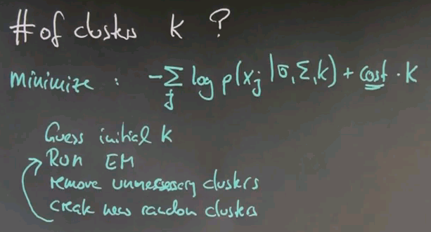
One of the remaining open questions pertains to the number of clusters. So far I've assumed it's simply constant and you know it. But in reality, you don't know it. Practical implementations often guess the number of clusters along with the parameters. And the way this works is that you periodically evaluate which data is poorly covered by the existing mixture, you generate new cluster centres at random near unexplained points, and then you run the algorithm for a while to see whether the existence of your clusters is still justified. And the justification test is based on a memorisation of a criterion that combines the negative log likelihood of your data itself and a penalty for each cluster. In particular, you're going to minimise the negative log likelihood of your data given the model plus a constant penalty per cluster.
If we look at this expression, this is the expression that EM already minimises. We maximised the posterior probability of data, logarithmic is a monotonic function, and I put a minus sign over here so the optimisation problem becomes a minimisation problem. This one over here, we have a constant cost per cluster, is new. If you increase the number of clusters, you would pay a penalty that is in the way of your attempted minimisation. Typically this expression balances out at a certain number of clusters, and it is generically the best explanation for your data.
So the algorithm looks as follows. Guess an initial K, run EM, remove unnecessary clusters that will make this cost over here go up, create some new random clusters, and go back and run EM.
There is all kinds of variants of this algorithm. One of the nice things here is this algorithm also overcomes local minima problems to some extent. If, for example, two clusters end up grabbing the same data, then your tests should show you that one of the clusters can be omitted; thereby the score can be improved. That cluster can later be restarted somewhere else, and by randomly restarting clusters, you tend to get a much, much better solution than if you run EM just once with a fixed number of clusters. So this trick is highly recommended for any implementation of expectation maximisation.
Clustering Summary
This finishes my unit on clustering. At least so far. I just want to briefly summarise what we've learned. We talked about k-means, and we talked about expectation maximisation. K-means is a very simple almost binary algorithm that allows you to find cluster centres. EM is a probabilistic generalisation that also allows you to find clusters but also modifies the shape of the clusters by modifying the covariance matrix. EM is probabilistically sound, and you can prove convergence in a log likelihood space. K-means also converges. Both are prone to local minima. In both cases you need to know the number of cluster centres, K. I showed you a brief trick how to estimate the K as you go which also overcomes local minima to some extent.
Dimensionality Reduction
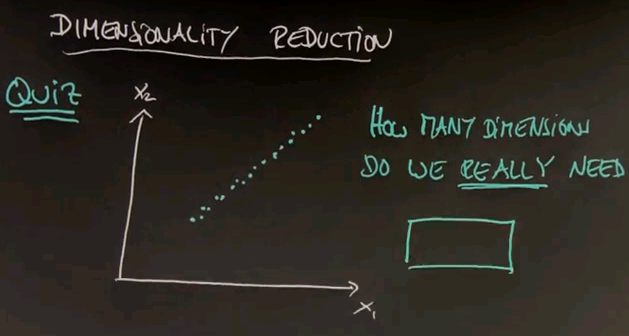
Let's now talk about a second class of unsupervised learning algorithms that are called dimensionality reduction. And I want to start with a little quiz, in which I will check your intuition. Suppose we're given a two-dimensional data field, and our data lines up as follows. My quiz is: How many dimensions do we really need? And the key is the work "really", which means we're willing to tolerate a certain amount of error in accuracy, because we want to capture the essence of the problem.
And the answer is obviously one. This is the key dimension over here. The orthogonal dimension in this direction carries almost no information so it suffices, in most cases, to project the data onto this one-dimensional space.
Question
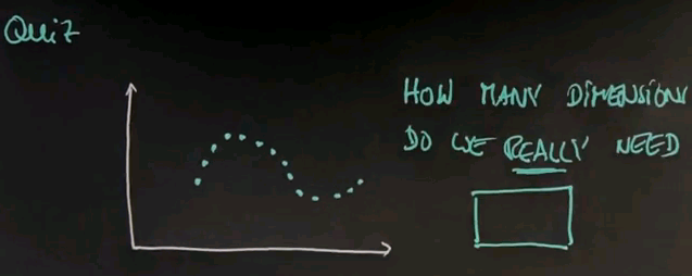
Here is a quiz that is a little bit more tricky. I'm going to draw data for you like this. I'm going to ask the same question. How many dimensions do we really need?
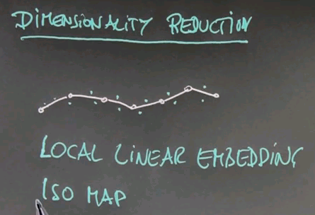
And this answer is not at all trivial, and I don't blame you if you get it wrong. The answer is actually 1, but the projection itself is nonlinear. I can draw, really easily, a nice 1-dimensional space that follows these data points. And if I'm able to project all the data points on this one-dimensional space, I capture the essence of the data. The trick of course is to find the nonlinear one-dimensional space and describe it. This is what's going on in the state-of-the-art in dimensionality reduction research.
Linear Dimensionality Reduction
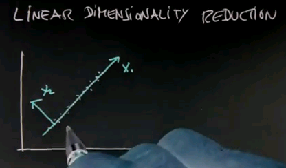
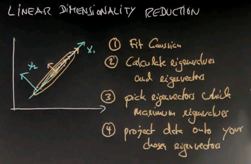
For the remainder of this unit, I'm going to talk about linear dimensionality reduction. Where the idea is that we're given data points like this, and we seek to find a linear subspace in which to project the data. In this case, I would submit this is probably the most suitable linear subspace. So we remap the data onto the space over here, with x1 over here and x2 over here. Then we can capture the data in just one dimension.
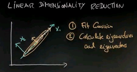
The algorithm is amazingly simple. Number 1: fit a Gaussian; we now know how this works. The Gaussian will look something like this. Number 2: calculate the eigenvalues and eigenvectors of this Gaussian. In this Gaussian this would be the dominant eigenvector, and this would be the second eigenvector over here.
Step 3 is take those eigenvectors whose eigenvalues are the largest, and step 4 is to project the data onto the subspace of the eigenvectors you chose.
Now to understand this, you have to be familiar with eigenvectors and eigenvalues. But I'll give you an intuitive familiarity with those. This is standard statistics material, and you will find this in many linear algebra classes. So let me just go through this very quickly and give you an intuition how to do linear dimensionality reduction.
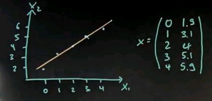
Suppose you're given the following data points. Your x's are 0, 1, 2, 3, and 4 for x1; and 1.9, 3.1, 4, 5.1 and 5.9. These are essentially 2, 3, 4, 5, 6; but slightly modified to define actual variance over this dimension. So we draw this in here. What I get is a set of points that doesn't quite fit a line, but almost.
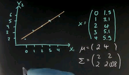
There's a little error over here, a little error over here, and here and here. Now the mean is easily calculated; it's 2 and 4. The covariance matrix looks as follows. Notice the slightly different covariance for the first variable, which is exactly 2, to the second variable, which is 2.008.
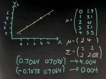
The eigenvectors happen to be 0.7064 and 0.7078 with an eigenvalue of 4.004. And the second one is orthogonal with an eigenvalue much smaller. So obviously this is the eigenvector that dominates the spread of the data points.
If you look at this vector over here, it is centred around the mean, which sits over here, and is exactly this vector shown over here. Whereas this one is the orthogonal vector, shown over here. So this is the single dimension with a large weight that explains the data relative to any other dimension, which is a very small eigenvalue.
I should mention why these numerical examples might look confusing. This is very standard linear algebra. When you estimate covariance from data and try to understand what direction they point, this kind of eigenvalue analysis gives you the right answer.
Face Example
The dimensionality reduction looks a little bit silly when we go from two dimensions to one dimension, but in truly high dimensional space it has a very strong utility. Here is an example that goes back to MIT several decades ago on something called eigenfaces.
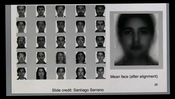
These are all well aligned faces and the objective in eigenface research has been to find simple ways to describe different people in a parameter space in which we can easily identify the same person again. Images like these are very high-dimensional statistics. If each images is fifty by fifty pixels, each image itself becomes a data point in a 2500 dimensional feature space. Now obviously we don't have random images. We don't fill the space of 2500 dimensions with all face images. Instead, it is reasonable to assume that all the faces line on a small subspace in that space. Obviously you as a human can easily distinguish what is a valid image of a face and what is a valid image of a non-face, like a car or a cloud or the sky. Therefore, there are many, many possible images that you can represent with 2500 pixels that are not faces. So research on eigenfaces has applied principle component analysis and eigenvalues to the space of faces. Here is a database in which faces are aligned, and a researcher at Santiago Serrano extracted from it the average face after alignment on the right side. The truly interesting phenomena occurs when you look at the eigenvalues.
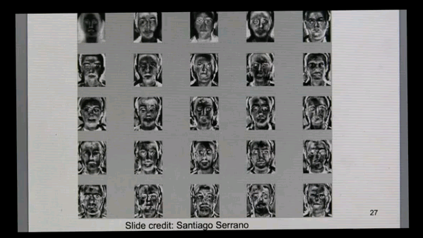
The face on the top left, over here, is the average face, and these are the variations, the eigenvectors that correspond to the largest eigenvalues over here. This is the strongest variation. You see a certain amount of different regions in and around the head shape and the hair that gets excited. That's the second strongest one, where the shirt gets more excited. And as you go down you find more and more interesting variations that can be used to reconstruct faces. Typically as dozen or so will suffice to make a face completely reconstructable. Which means we've just mapped a 2500 dimensional feature space into a perhaps 12 dimensional feature space on which we can now learn much, much easier.
Scan Example
In our own research, we also have applied eigenvector decomposition to relatively challenging problems that don't look like a linear problem at the surface. We scanned a good number of people with different physiques: some thin, some not so thin, some tall, some short, some male, some female. And we also scanned them in 3D in different body postures: the arms down, the arms up, walking, throwing a ball, and so on. And we applied eigenvector decomposition to the type I've just shown you to understand whether there is a latent low-dimensional space that is sufficient to represent the different physiques that people have, like thin or thick, and the different postures people can assume, like standing and so on. It turns out if you apply eigenvector decomposition to the space of all the formations of your body, you can find relatively low dimensional linear spaces, in which you can express different physiques and different body postures. For the space of all different physiques it turned out only three dimensions sufficed to explain different heights, different thicknesses or body weights, and also different genders. That is, even though our surfaces themselves are representative of tens of thousands of data points, the underlying dimensionality when scanning people is really small. I'll let you watch the entire movie. Please enjoy.
SCAPE: Shape Completion and Animation of People.
Piece-Wise Linear Projection
In modern dimensionality reduction, the trick has been to define nonlinear, sometimes piece-wise linear, subspaces on which data is being projected. This is not dissimilar from k nearest neighbours, where local regions are being defined based on local data neighbourhoods. But here we need ways to interpret leveraging neighbours to make sure that the subspace itself becomes a feasible subspace.
Common methods include local linear embedding, or LLE, or the ISO map method. If you're interested in this, check the web. There's tons of information on these methods on the world wide web.
Spectral Clustering
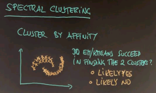
I will now talk about spectral clustering. The fundamental idea of spectral clustering is to cluster by affinity. And to understand the importance of spectral clustering, let me ask you a simple intuitive quiz. Suppose you are given data like this, and you wish to learn that there's two clusters -- a cluster over here and a cluster over here. So my question is, from what you understand, do you think that EM or k-means would do a great job finding those clusters or do you think they will likely fail to find those clusters?
So the questions: Do EM or k-means succeed in finding the two clusters? There's a likely yes, and a likely no.
And the answer is likely no. The reason being that these aren't clusters defined by a centre of data points, but they're clusters defined by affinity, which means they're defined by the presence of nearby points. So take for example the area over here, which I'm going to circle, and ask yourself, what's the best cluster centre? It's likely somewhere over here where I drew the red dot. This is the cluster centre for this cluster, and perhaps this is the cluster centre for the other cluster, and these points over here will likely be classified as belonging to the cluster centre over here. So EM will likely do a bad job.
Spectral Clustering Algorithm
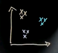
So let's look at this example again -- let me redraw the data. What makes these clusters so different is not the absolute location of each data point, but the connectedness of these data points. The fact that these two points belong together is likely because there's lots of points in between. In other words, it's the affinity that defines those clusters, not the absolute location. So spectral clustering gets a notion of affinity to make clustering happen.
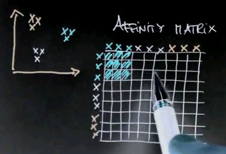
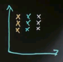
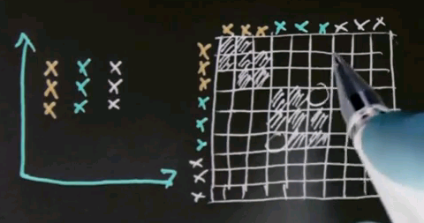
So let me look at the simple example for spectral clustering that would also work for k-means or EM but that'll be useful to illustrate spectral clustering. Let's assume there's nine data points as shown over here, and I've coloured them differently in blue, red and black. But to clustering algorithms, they all come with the same colour.
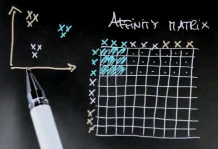
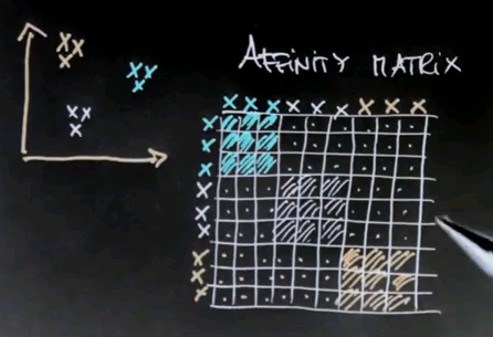
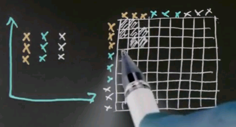
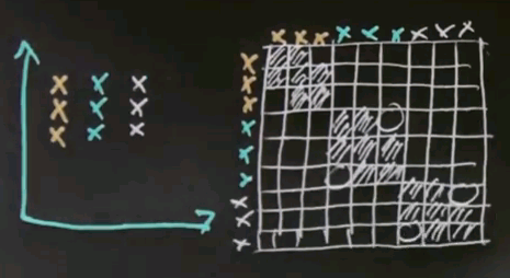
Now the key element of spectral clustering is called the affinity matrix, which is a 9x9 matrix in this case, where each data point gets graphed relative to each other data point. So let me write down all the nine data points into the different rows of this matrix -- the red ones, the black ones, and the blue ones. And in the columns, I graphed the exact same nine data points. I then calculate for each pair of data points their affinity, where I use for now affinity as the quadratic distance in this diagram over here. Clearly the red dots to each other have high affinity, which means a small quadratic distance. Let me indicate this as follows.
But relative to all the other points, the affinity is weak. So there is a very small affinity in these elements over here.
Similarly, the affinity of the black data points to each other is very high, which means that the following block diagonal in this matrix will have a very large value. Yet the affinity to all other data points will be low. And of course, the same is true for the blue data points.
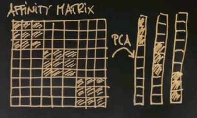
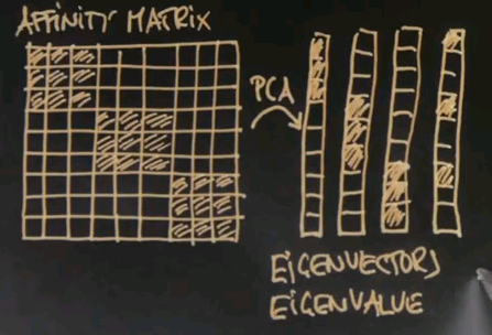
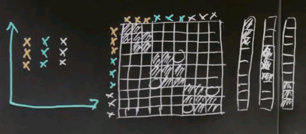
The interesting thing to notice now is that this is an approximately rank-deficient matrix. And further, the data points that belong to the same class -- like the three red dots or the three black dots -- have a singular affinity vector to all the other data points. So this vector over here is similar to this vector over here. It's similar to this vector over here, but it's very different to this vector over here, which then itself is similar to the vector over here, yet different to the previous ones. Such a situation is easily addressed by what's called principle component analysis, or PCA. PCA is a method to identify vectors that are similar in an approximate rank-deficient matrix.
Consider once again our affinity matrix. With principle component analysis, which is a standard linear trick, we can re-represent this matrix by the most dominant vectors you'll find there. And the first one might look like this. The second one, which would be orthogonal, may look like this. The third one, like this.
These are called eigenvectors, and in principle component analysis each component vector has an eigenvalue that states how prevalent this vector is in the original data. And for these three vectors you're going to find a large eigenvalue because there's a number of data points that represent these vectors quite prevalently like the first three does for this guy over here. There might be additional eigenvectors, like something like this.
But such eigenvectors will have a small eigenvalue simply because this vector isn't really required to explain the data over here. It might just be explaining some of the noise in the affinity matrix that I didn't even dare draw in here. Now if you take the eigenvectors with the largest eigenvalues, three in this case, you first discover that the dimensionality of the underlying data space. The dimensionality equals the number of large eigenvalues. Futher, if you re-represent each data vector using those eigenvectors, you'll find a three-dimensional space where original data falls into a variety of different places. And these places are easily told apart by conventional clustering. So in summary, spectral clustering builds an affinity matrix of the data points, extracts the eigenvectors with the largest eigenvalues, and then re-maps those vectors into a new space where the data points easily cluster in the conventional way. This is called affinity based clustering or spectral clustering.
Let me illustrate this once again with a data set that has a different spectral clustering than a conventional clustering. In this data set, the different clusters belong together because their affinity is similar. These two points belong together because their is a point in between.
If we now draw the affinity matrix for those data points, you find that the first and second data points are close together and the second and the third, but not the first and the third. Hence these two off diagonal elements here have remained small.
Similarly for the red points as shown here where these two elements over here are relatively small.
And also for the black points where these two elements over here are small.
And interestingly enough, even though these aren't block diagonal, your first three largest eigenvectors will still look the same as before.
I find this quite remarkable that even though these aren't exactly blocks, those vectors still represent the three most important vectors for which to recover the data using principle component analysis. So in this case spectral clustering would easily assign those guys and those guys and those guys to the respective same cluster, which wouldn't be quite as easily the case for expectation maximisation or k-means.
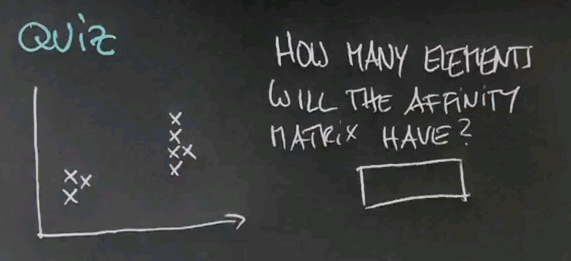
So let me ask you the following quiz. Suppose we have eight data points. How many elements will the affinity matrix have?
And the answer is 64. There's eight data points -- 8 times 8 is 64.
Question
My second question is, how many large eigenvalues will PCA find? Now I understand this doesn't have a unique answer, but in the best possible case, where spectral clustering works well, how many large eigenvalues do you find?
There's a cluster over here and a cluster over here. And while it might happen that it's as many as eight, if you adjust your affinity matrix well, those two should correspond with the two largest eigenvalues.
Supervised vs Unsupervised Learning
So, congratulations. You just made it through the unsupervised learning section of this class. I think you've learned a lot. You learned about k-means, you learned about expectation maximisation, about dimensionality reduction and even spectral clustering. The first three algorithms -- k-means, EM and dimensionality reduction -- are used very frequently, and spectral clustering is a rarer used method that shows some of the most recent research going on in the field. I hope you have fun applying these methods in practice.
I'd like to say a few final words about supervised versus unsupervised learning. In both cases you're given data, but in one case you have labelled data, in another you have unlabelled data. The supervised learning paradigm is the dominant paradigm in machine learning, and the vast amount of papers being written about it. We talked about classification and regression and different methods to do supervised learning. The unsupervised paradigm is much less explored, even though I think it's at least equally important -- possibly even more important. Many systems can collect vast amounts of data such as web crawlers, robots, I told you about Street View, and getting the data is cheap, but getting labels is hard. So to me, unsupervised is the method of the future. It's one of the most interesting open research topics to see whether we can make sense out of large amounts of unlabelled or poorly labelled data. Now in between, there are techniques that do both: supervised and unsupervised. They are called semi-supervised or self-supervised, and they use elements of unsupervised learning and pair them with supervised learning. Those are fascinating by their own rights. Our robot Stanley, for example, that won the DARPA Grand Challenge, used its own sensors to produce labels on the fly to other data. And I talked about this when I talk about robotics in more detail. But for the time being, understand that the paradigms supervised and unsupervised spam two very large areas of machine learning, and you learned quite a bit about it.
