AI class unit 5
These are my notes for unit 5 of the AI class.
Machine Learning
Introduction
Welcome to the machine learning unit. Machine learning is a fascinating area. The world has become immeasurably data-rich. The world wide web has come up over the last decade. The human genome is being sequenced. Vast chemical databases, pharmaceutical databases, and financial databases are now available on a scale unthinkable even five years ago. To make sense out of the data, to extract information from the data, machine learning is the discipline to go.
Machine learning is an important sub-field of artificial intelligence, it's my personal favourite next to robotics because I believe it has a huge impact on society and is absolutely necessary as we move forward.
So in this class, I teach you some of the very basics of machine learning, and in our next unit Peter will tell you some more about machine learning. We'll talk about supervised learning, which is one side of machine learning, and Peter will tell you about unsupervised learning, which is a different style. Later in this class we will also encounter reinforcement learning, which is yet another style of machine learning. Anyhow, let's just dive in.
What is Machine Learning?
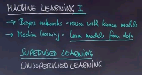
Welcome to the first class on machine learning. So far we talked a lot about Bayes Networks. And the way we talked about them is all about reasoning within Bayes Networks that are known. Machine learning addresses the problem of how to find those networks or other models based on data. Learning models from data is a major, major area of artificial intelligence and it's perhaps the one that had the most commercial success. In many commercial applications the models themselves are fitted based on data. For example, Google uses data to understand how to respond to each search query. Amazon uses data to understand how to place products on their website. And these machine learning techniques are the enabling techniques that make that possible.
So this class which is about supervised learning will go through some very basic methods for learning models from data, in particular, specific types of Bayes Networks. We will complement this with a class on unsupervised learning that will be taught next after this class.
Let me start off with a quiz. The quiz is: What companies are famous for machine learning using data? Google for mining the web. Netflix for mining what people would like to rent on DVDs. Which is DVD recommendations. Amazon.com for product placement. Check any or all and if none of those apply check down here.
And, not surprisingly, the answer is all of those companies and many, many more use massive machine learning for making decisions that are really essential to their businesses. Google mines the web and uses machine learning for translation, as we've seen in the introductory level. Netflix has used machine learning extensively for understanding what type of DVD to recommend to you next. Amazon composes its entire product pages using machine learning by understanding how customers respond to different compositions and placements of their products, and many, many other examples exist. I would argue that in Silicon Valley, at least half the companies dealing with customers and online products do extensively use machine learning. So it makes machine learning a really exciting discipline.
Stanley DARPA Grand Challenge
In my own research, I've extensively used machine learning for robotics. What you see here is a robot my students and I built at Stanford called Stanley, and it won the DARPA Grand Challenge. It's a self-driving car that drives without any human assistance whatsoever, and this vehicle extensively uses machine learning.
The robot is equipped with a laser system. I will talk more about lasers in my robotics class, but here you can see how the robot is able to build 3D models of the terrain ahead. These are almost like video game models that allow it to make assessments where to drive and where not to drive. Essentially it's trying to drive on flat ground.
The problem with these lasers is that they don't see very far. They only see about 25 meters out, so to drive really fast the robot has to see further, and this is where machine learning comes into play. What you see here is camera images delivered by the robot superimposed with laser data that doesn't see very far, but the laser is good enough to extract samples of driveable road surface that can then be machine learned and extrapolated into the entire camera image. That enables the robot to use the camera to see driveable terrain all the way to the horizon up to like 200 meters out, enough to drive really, really fast. This ability to adapt its vision by driving its own training examples using lasers but seeing out 200 meters or more was a key factor in winning the race.
Taxonomy
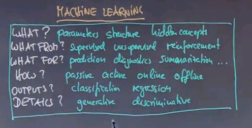
Machine learning is a very large field with many different methods and many different applications. I will now define some of the very basic terminology that is being used to distinguish different machine learning methods.
Let's start with the what. What is being learned? You can learn parameters like the probabilities of a Bayes Network. You can learn structure like the arc structure of a Bayes Network. And you might even discover hidden concepts. For example, you might find that certain training examples form a hidden group. For example, Netflix might find that there's different types of customers some that care about classic movies some of them care about modern movies and those might form hidden concepts whose discovery can really help you make better sense of the data.
Next is what from? Every machine learning method is driven by some sort of target information that you care about. In supervised learning which is the subject of today's class we're given specific target labels and I'll give you examples in just a second. We also talk about unsupervised learning where target labels are missing and we use replacement principles to find, for example hidden concepts. Later there will be a class on reinforcement learning when an agent learns from feedback with the physical environment by interacting and trying actions and receiving some sort of evaluation from the environment like "Well done" or "That works." Again, we will talk about those in detail later.
There's different things you could try to do with machine learning techniques. You might care about prediction. For example you might want to care about what's going to happen with the future in the stockmarket for example. You might care to diagnose something which is you get data and you wish to explain it and you use machine learning for that. Sometimes your objective is to summarise something. For example if you read a long article your machine learning method might aim to produce a short article that summarises the long article. And there's many, many, many more different things.
You can talk about the how to learn. We use the word passive if your learning agent is just an observer and has no impact on the data itself. Otherwise we call it active. Sometimes learning occurs online which means while the data is being generated and some of it is offline which means learning occurs after the data has been generated.
There's different types of outputs of a machine learning algorithm. Today we'll talk about classification versus regression. In classification the output is binary or a fixed number of classes for example something is either a chair or not. Regression is continuous. The temperature might be 66.5 degrees in our prediction.
And there's tons of internal details we will talk about. Just to name one. We will distinguish generative from discriminative. Generative seeks to model the data as generally as possible versus discriminative methods seek to distinguish data and this might sound like a superficial distinction but has enormous ramification on the learning algorithm.
Now to tell you the truth it took me many years to fully learn all these words here and I don't expect you to pick them all up in one class but you should as well know that they exist. And as they come up I'll emphasise them so you can resort any learning method I tell you back into the specific taxonomy over here.
Supervised Learning
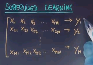
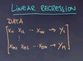
The vast amount of work in the field falls into the area of supervised learning. In supervised learning you're given for each training example a feature vector and a target label named Y. For example, for a credit rating agency X1, X2, X3 might be a feature such as is the person employed? What is the salary of the person? Has the person previously defaulted on a credit card? And so on. And Y is a predictor whether the person is to default on the credit or not. Now machine learning is typically carried out on past data where the credit rating agency might have collected features just like these and actual occurrences of default or not. What it wishes to produce is a function that allows us to predict future customers. So when a new person comes in with a different feature vector, can we predict as good as possible the functional relationship between these features X1 to Xn all the way to Y? You can apply the exact same example in image recognition where X might be pixels of images or it might be features of things found in images and Y might be a label that says whether a certain object is contained in an image or not.
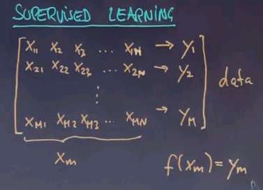
Now in supervised learning you're given many such examples. X21 to X2n leads to Y2 all the way to index m.
This is called your data. If we call each input vector Xm and we wish to find out the function given any Xm or any future vector X produces as close as possible my target signal Y. Now this isn't always possible and sometimes it's acceptable, in fact preferable, to tolerate a certain amount of error in your training data. But the subject of machine learning is to identify this function over here.
And once you identify it you can use it for future Xs that weren't part of the training set to produce a prediction that hopefully is really, really good.
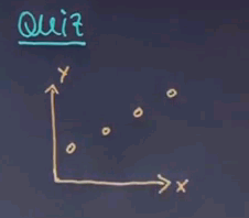
So let me ask you a question. And this is a question for which I haven't given you the answer but I'd like to appeal to your intuition. Here's one data set where the X is one dimensionally plotted horizontally and the Y is vertically and suppose that looks like this.
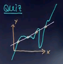
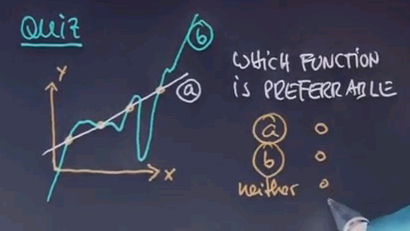
Suppose my machine learning algorithm gives me two hypotheses. One is this function over here which is a linear function and one is this function over here.
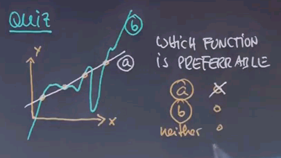
I'd like to know which of the functions you find preferable as an explanation for the data. Is it function A? Or function B?
Occam's Razor
And I hope you guessed function A. Even though both perfectly describe the data B is much more complex than A. In fact, outside the data B seems to go to minus infinity much faster than these data points and to plus infinity much faster than with these data points over here. And in between we have wild oscillations that don't correspond to any data. So I would argue A is preferable.
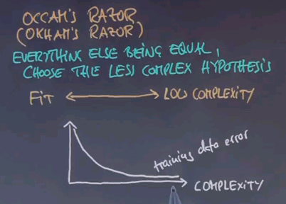
The reason why I asked this question is because of something called Occam's Razor. Occam can be spelled many different ways. And what Occam says is that everything else being equal choose the less complex hypothesis.
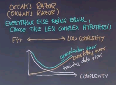
Now in practice there's actually a trade-off between a really good data fit and low complexity. Let me illustrate this to you by a hypothetical example. Consider the following graph where the horizontal axis graphs complexity of the solution. For example, if you use polynomials this might be a high-degree polynomial over here and maybe a linear function over here which is a low-degree polynomial. Your training data error tends to go like this.
The more complex the hypothesis you allow the more you can just fit your data. However, in reality your generalisation error on unknown data tends to go like this. It is the sum of the training data error and another function which is called the overfitting error.
Not surprisingly the best complexity is obtained where the generalisation error is minimum. There are methods to calculate the overfitting error. They go into a statistical field under the name Bayes variance methods. However, in practice you're often just given the training data error. You find if you don't find the model that minimises the training data error but instead pushes back the complexity your algorithm tends to perform better and that is something we will study a little bit in this class.
However, this slide is really important for anybody doing machine learning in practice. If you deal with data and you have ways to fit your data be aware that overfitting is a major source of poor performance of a machine learning algorithm. And I'll give you examples in just one second.
SPAM Detection
So a really important example of machine learning is SPAM detection. We all get way too much email and a good number of those are SPAM. Here are three examples of email. "Dear Sir: First I must solicit your confidence in this transaction, this is by virtue of its nature as being utterly confidential and top secret..." This is likely SPAM. Here's another one, in upper caps. "99 MILLION EMAIL ADDRESSES FOR ONLY $99" This is very likely SPAM. And here's another one. "Oh, I know this is blatantly OT but I'm beginning to go insane. Had an old Dell Dimension XPS sitting in the corner and decided to put it to use. I know it was working pre being stuck in the corner, but when I plugged it in, hit the power nothing happened." Now this is likely not SPAM.
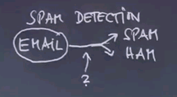
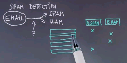
How can a computer program distinguish between SPAM and not SPAM? Let's use this as an example to talk about machine learning for discrimination using Bayes Networks. In SPAM detection we get an email and we wish to categorise it either as SPAM in which case we don't even show it to the reader or what we call HAM which is the technical word for an email worth passing on to the person being emailed. So the function over here is the function we're trying to learn.
Most SPAM filters use human input. When you go through your email you have a button called "IS SPAM" which allows you as a user to flag SPAM and occasionally you will say an email is SPAM. If you look at this you have a typical supervised machine learning situation where the input is an email and the output is whether you flag it as SPAM or if we don't flag it we just think it's HAM.
Now to make this amenable to a machine learning algorithm we have to talk about how to represent emails. They're all using different words and different characters and they might have different graphics included. Let's pick a representation that's easy to process. And this representation is often called Bag of Words. Bag of Words is a representation of a document that just counts the frequency of words. If an email were to say "Hello I will say Hello." The Bag of Words representation is the following.
2-1-1-1 for the dictionary that contains the four words "Hello", "I", "will", "say". Now look at the subtlety here. Rather than representing each individual word we have a count of each word and the count is oblivious to the order in which the words were stated. A Bag of Words representation relative to a fixed dictionary represents the counts of each word relative to the words in the dictionary.
If you were to use a different dictionary like "Hello" and "Good-bye" our counts would be 2 and 0. However, in most cases you make sure that all the words found in messages are actually included in the dictionary. So the dictionary might be very, very large.
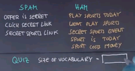
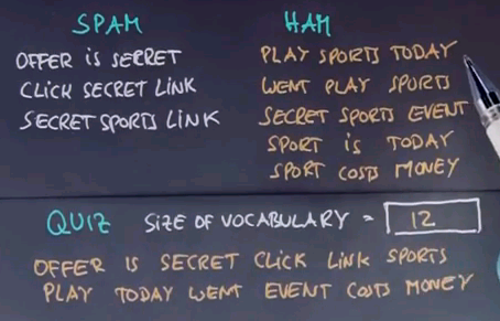
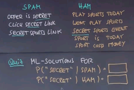
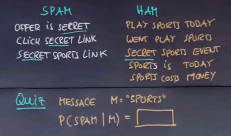
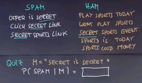
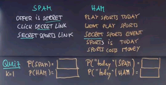
Let me make up an unofficial example of a few SPAM and a few HAM messages. "Offer is secret". "Click secret link". "Secret sports link". Obviously those are contrived and I tried to retain the vocabulary to a small number of words to make this example workable. In practice we need thousands of such messages to get good information. "Play sports today". "Went play sports". "Secret sports event". "Sport is today". "Sport costs money". My first quiz is: what is the size of the vocabulary that contains all words in these messages? Please enter the value in this box over here.
Well let's count. "Offer", "is", "secret", "click". "Secret" occurs over here already so we don't have to count it twice. "Link", "sports", "play", "today", "went", "event", "costs", "money". So the answer is 12. There's twelve different words contained in these eight messages.
Question
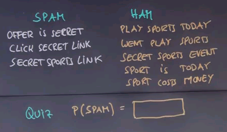
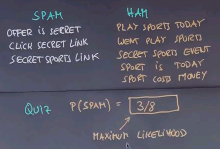
Another quiz. What is the probability that a random message that arrives will fall into the spam bucket? Assuming that those messages are all drawn at random.
And the answer is: there's eight different messages of which three are spam. So the maximum likelihood estimate is 3/8.
Maximum Likelihood
Note: Assume the question is asking for the probability of a word in a spam message being "secret" NOT the probability that a spam message contains the word secret.
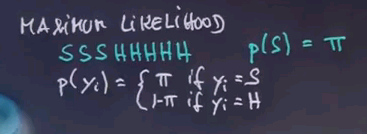
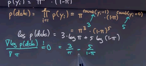
So, let's look at this a little bit more formally and talk about maximum likelihood. Obviously, we're observing eight messages: spam, spam, spam and five times ham. And what we care about is what's our prior probability of spam that maximises the likelihood of this data?
So, let's assume we're going to assign a value of pi to this, and we wish to find the pi that maximises the likelihood of this data over here, assuming that each email is drawn independently according to an identical distribution. The probability of the p(yi) data item is then pi if yi = spam, and 1 - pi if yi = ham.
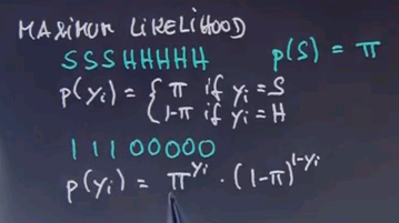
If we rewrite the data as 1,1,1,0,0,0,0,0, we can write p(yi) as follows: pi to the yi times (1 - pi) to the 1 - yi.
It's not that easy to see that this is equivalent, but say yi = 1. Then this term will fall out. It's a multiplication by 1 because the exponent is zero, and we get pi as over here. If yi = 0, then this term falls out, and this one here becomes 1 - pi as over here.
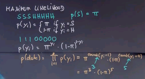
Now assuming independence, we get for the entire data set that the joint probability of all data items is the product of the individual data items over here, which can now be written as follows:
pi to the count of instances where yi = 1 times 1 - pi to the count of the instances where yi = 0. And we know in our example, this count over here is three, and this count over here is five, so we get pi to the third times 1 - pi to the fifth.
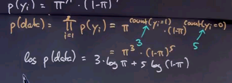
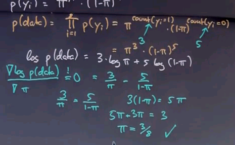
We now wish to find the pi that maximises this expression over here. We can also maximise the logarithm of this expression, which is three times log pi + five times log (1 - pi).
Optimising the log is the same as optimising p because the log is monotonic in p. The maximum of this function is attained with a derivative of zero, so let's compute with a derivative and set it to zero. This is the derivative, 3 over pi - 5 over 1 - pi.
We now bring this expression to the right side, multiply the denominators up, and sort all the expressions containing pi to the left, which gives us pi = 3/8, exactly the number we were at before.
So we just derived mathematically that the data likelihood maximising number for the probability is indeed the empirical count, which means when we looked at this quiz before and we said a maximum likelihood for the prior probability of spam is 3/8, by simply counting 3 over 8 emails were spam, we actually followed proper mathematical principles to do maximum likelihood estimation. Now, you might not fully have gotten the derivation of this, and I recommend you to watch it again, but it's not that important for the progress in this class.
So, here's another quiz. I'd like the maximum likelihood, or ML solutions, for the following probabilities. The probability that the word "secret" comes up, assuming that we already know a message is spam, and the probability that the same word "secret" comes up if we happen to know the message is not spam, it's ham.
And just as before we count the word secret in SPAM and in HAM as I've underlined here. Three out of nine words in SPAM are the word "secret" so we have a third over here, or 0.333, and only one out of all the fifteen words in HAM are "secret" so you get a fifteenth or 0.0667.
Relationship to Bayes Networks
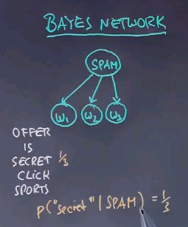
By now, you might have recognised what we're really building up is a Bayes network where the parameters of the Bayes networks are estimated using supervised learning by a maximum likelihood estimator based on training data.
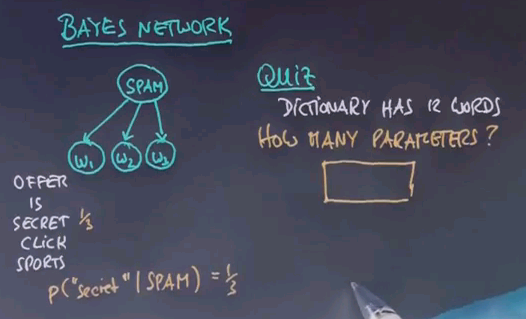
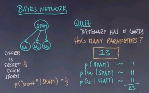
The Bayes network has at its root an unobservable variable called spam, which is binary, and it has as many children as there are words in a message, where each word has an identical conditional distribution of the word occurrence given the class spam or not spam. If you write down our dictionary over here -- you might remember the dictionary had twelve different words -- so here is five of the twelve, "offer", "is", "secret", "click" and "sports". Then for the spam class, we found the probability of "secret" given spam is 1/3, and we also found that the probability of "secret" given ham is 1/15.
So here's a quiz. Assuming a vocabulary size of twelve, or put differently, the dictionary has twelve words, how many parameters do we need to specify this Bayes network?
And the correct answer is 23. We need one parameter for the prior p(spam), and then we have two dictionary distributions of any word i given spam, and the same for ham. Now, there's twelve words in a dictionary, but this distribution only needs eleven parameters, so twelve can be figured out because they have to add up to 1. And the same is true over here, so if you add all these together, we get 23.
Question
So, here's a quiz. Let's assume we fit all the 23 parameters of the Bayes network as explained using maximum likelihood. Let's now do classification and see what class and message it ends up with. Let me start with a very simple message, and it contains a single word just to make it a little bit simpler. What's the probability that we classify this one word message as spam?
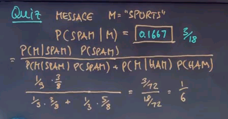
And the answer is 0.1667 or 3/18.
How do I get there? Well, let's apply Bayes rule. This form is easily transformed into this expression over here, the probability of the message given spam times the prior probability of spam over the normaliser over here. Now, we know that the word "sports" occurs 1 in our 9 words of spam, and our prior probability for spam is 3/8, which gives us this expression over here. We now have to add the same probabilities for the class ham. Sports occurs 5 times out of 15 in the ham class, and the prior probability for ham is 5/8, which gives us 3/72 divided by 18/72, which is 3/18 or 1/6.
Question
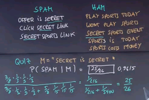
Let's do a more complicated quiz. Say the message now contains 3 words. "Secret is secret", not a particularly meaningful email, but the frequent occurrence of "secret" seems to suggest it might be spam. So what's the probability you're going to judge this to be spam?
And the answer is surprisingly high. It's 25/26, or 0.9615. To see if we apply Bayes rule, which multiplies the prior for spam-ness with the conditional probability of each word given spam. "Secret" carries 1/3, "is" 1/9, and "secret" 1/3 again. We normalise this by the same expression plus the probability for the non-spam case. 5/8 as a prior. "Secret" is 1/15. "Is" is 1/15, and "secret" again. This resolves to 1/216 over this expression plus 1/5400, and when you work it all out is 25/26.
Question
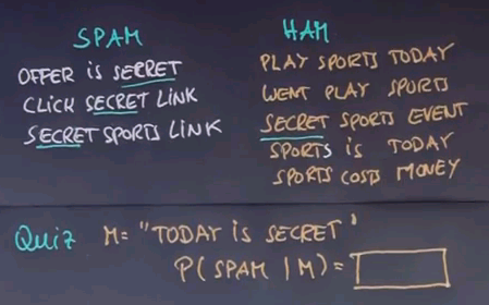
A final quiz. Let's assume our message is "Today is secret". Again, it might look like spam because the word "secret" occurs. I'd like you to compute for me the probability of spam given this message.
Answer and Laplace Smoothing
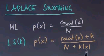
Note: At 2:20: count(x) is the number of occurrences of this value of the variable x. |x| is the number of values that the variable x can take on. k is a smoothing parameter. And N is the total number of occurrences of x (the variable, not the value) in the sample size.
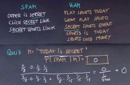
And surprisingly, the probability for this message to be spam is 0. It's no 0.001. It's flat 0. In other words, it's impossible, according to our model, that this text could be a spam message. Why is this? Well when we apply the same rule as before, we get the prior for spam which is 3/8. And we multiply the conditional for each word into this. For "secret", we know it to be 1/3. For "is", to be 1/9, but for "today", it's 0. It's zero because the maximum of the estimate for the probability of "today" in spam is zero. "Today" just never occurred in a spam message so far. Now, this 0 is troublesome because as we compute the outcome -- and I'm plugging in all the numbers as before -- none of the words matter anymore, just the zero matters. So we get zero over something which is plain zero. Are we overfitting? You bet. We are clearly overfitting.
It can't be that a single word determines the entire outcome of our analysis. The reason is that our model, to assign a probability of zero for the word "today" to be in the class of spam is just too aggressive. So let's change this.
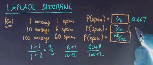
One technique to deal with the overfitting problem is called Laplace Smoothing. In maximum likelihood estimation, we assign towards our probability the quotient of the count of this specific event over all events in our data set. So for example, for the prior probability, we found that 3/8 messages are spam. Therefore, our maximum likelihood estimate for the prior probability of spam was 3/8. In Laplace Smoothing, we use a different estimate. We add the value k to the count and normalise as if we added k to every single class that we've tried to estimate something over.
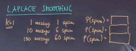
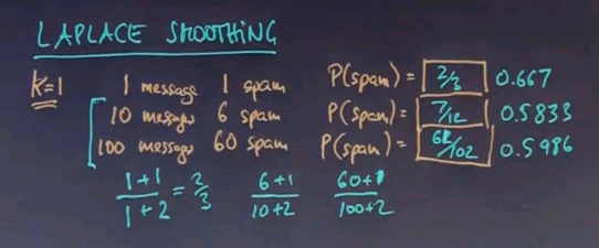
This is equivalent to assuming we have a couple of fake training examples where we add k to each observation count. Now, if k equals 0, we get our maximum likelihood estimator. But if k is larger than 0 and n is finite, we get different answers. Let's set k equals 1, and let's assume we get one message, and that message was spam, so we're going to write it one message, one spam. What is p(spam) for the Laplace smoothing of k + 1? Let's do the same with 10 messages, and we get 6 spam. And 100 messages, of which 60 are spam. Please enter your numbers into the boxes over here.
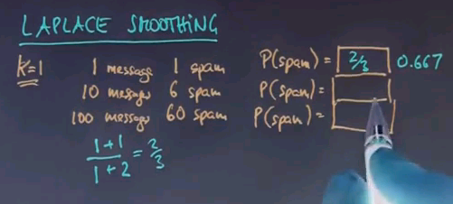
The answer here is 2/3 or 0.667 and is computed as follows. We have 1 message with 1 as spam, but we're going to add k = 1. We're going to add k = 2 over here because there's 2 different classes. k = 1 times 2 equals 2, which gives us 2/3.
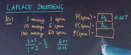
The answer over here is 7/12. Again, we have 6/10 but we add 2 down here and 1 over here, so you get 7/12.
And correspondingly, we get 61/102 is 60 + 1 over 100 + 2.
If we look at the numbers over here, we get 0.5833 and 0.5986.
Interestingly, the maximum likelihood on the last 2 cases over here will give us 0.6, but we only get a value that's closer to 0.5, which is the effect of our smoothing prior for the Laplacian smoothing.
Question
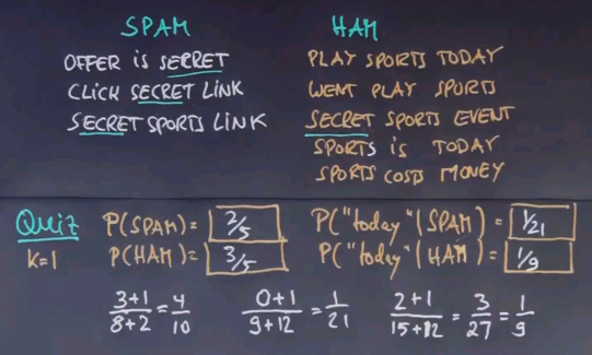
Let's use the Laplacian smoother with k=1 to calculate a few interesting probabilities -- P(SPAM) and P(HAM) -- and then the probability of the words "today", given that it's in the SPAM class or the HAM class. And you might assume that our vocabulary size is about 12 different words here.
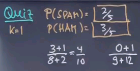
This one is easy to calculate for SPAM and HAM. For SPAM it's 2/5, and the reason is, we had previously 3 out of 8 messages assigned to SPAM, but thanks to the Laplacian smoother we add 1 over here, and there are 2 classes, so we add 2 times 1 over here, which gives us 4/10, which is 2/5.
Similarly we get 3/5 over here. Now the tricky part comes up over here. Before we had 0 occurrences of the word "today" in the SPAM class, and we had 9 data points. But now we're going to add 1 for Laplacian smoother, and down here we're going to add 12.
And the reason that we add 12 is because there's 12 different words in our dictionary. Hence, for each word in the dictionary we are going to add 1. So we have a total of 12, which gives us the 12 over here. That makes 1/21.
In the HAM class, we had 2 occurrences of the word "today" -- over here and over here. We add 1, normalise by 15, plus 12 for the dictionary size, which is 3/27 or 1/9.
This was not an easy question.
Question
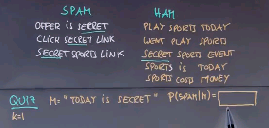
We come now to the final quiz here, which is -- I would like to compute the probability that the message "today is secret" falls into the SPAM box with Laplacian smoother using k=1. Please just enter your number over here. This is a non-trivial question. It might take you a while to calculate this.
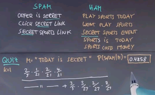
And the approximate probability is 0.4858. How did we get this? Well, the prior probability for SPAM under the Laplacian smoothing is 2/5. "Today" doesn't occur, but we have already calculated this to be 1/21. "Is" occurs once, so we get 2 over here over 21. "Secret" occurs 3 times, so we get a 4 over here over 21, and we normalise this by the same expression over here, plus the prior for HAM, which is 3/5, we have 2 occurrences of "today", plus 1, equals 3/27. "Is" occurs once for 2/27. And "secret" occurs once, again, 2/27. When you work this all out, you get this number over here.
Summary Naive Bayes
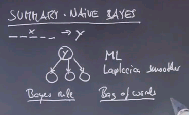
So we learned quite a bit. We learned about Naive Bayes as our first supervised learning method. The setup was that we had features of documents or training examples. And labels, in this case, SPAM or not SPAM. And from those features we made a generative model for the SPAM class and the non-SPAM class that described the conditional probability of each individual feature. We then used first maximum likelihood and then a Laplacian smoother to fit those parameters over here. And then using Bayes rule we could take any training example over here and figure our what the class probability was over here. This is called a generative model in that the conditional probabilities all aim to maximise the probability of individual features as if those describe the physical world. We also used what's called a bag of words model, in which our representation of each email was such that we just counted the occurrences of words, irrespective of their order.
Now this is a very powerful method for fighting SPAM. Unfortunately, it's not powerful enough. It turns out spammers know about Naive Bayes, and they've long learned to come up with messages that are fooling your SPAM filter if it uses Naive Bayes. So companies like Google and others have become much more involved in methods for SPAM filtering. Now I can give you some more examples how to filter SPAM, but all of those quite easily fit with the same Naive Bayes model.
Advanced SPAM Filtering
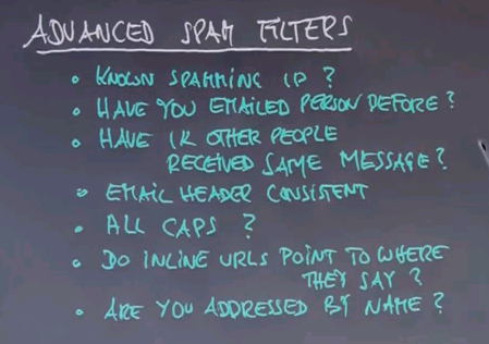
So here are features that you might consider when you write an advanced spam filter. For example, does the email come from a known spamming IP or computer? Have you emailed this person before? In which case it is less likely to be spam. Here's a powerful one: have 1000 other people recently received the same message? Is the email header consistent? So for example if the from field says your bank is the IP address really your bank? Surprisingly is the email all caps? Strangely many spammers believe if you write things in all caps you'll pay more attention to it. Do the inline URLs point to those pages where they say they're pointing to? Are you addressed by your correct name?
Now these are some features, I'm sure you can think of more. You can toss them easily into the Naive Bayes model and get better classification. In fact modern spam filters keep learning as people flag emails as spam and of course spammers keep learning as well and trying to fool modern spam filters. Who's going to win? Well so far the spam filters are clearly winning. Most of my spam I never see, but who knows what's going to happen in the future..? It's a really fascinating machine learning problem.
Digit Recognition
Naive Bayes can also be applied to the problem of hand written digit recognition. This is a sample of hand-written digits taken taken from a U.S. postal data set where hand written zip codes on letters are being scanned and automatically classified.
The machine learning problem here is taking a symbol just like this, what is the corresponding number? Here it's obviously 0. Here it's obviously 1. Here it's obviously 2, 1. For the one down here it's a little bit harder to tell.
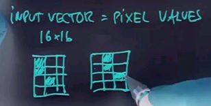
Now when you apply Naive Bayes, the input vector could be the pixel values of each individual pixel, so we have a 16 x 16 input resolution. You would get 156 different values corresponding to the brightness of each pixel. Now obviously given sufficiently many training examples you might hope to recognise digits, but one of the deficiencies of this approach is it's not particularly shift-invariant.
So, for example, a pattern like this will look fundamentally different from a pattern like this:
Even though the pattern on the right is obtained by shifting the pattern on the left by 1 to the right. There's many different solutions, but a common one could be to use smoothing in a different way from the way we discussed it before. Instead of just counting 1 pixel value's count, you could mix it with the counts of the neighbouring pixel values so if all pixels are slightly shifted, we get about the same statistics as the pixel itself. Such a method is called input smoothing. You can what's technically called convolve the input vector with the Gaussian variable, and you might get better results that if you do Naive Bayes on the raw pixels. Now to tell you the truth for digit recognition of this type, Naive Bayes is not a good choice. The conditional independence assumption of each pixel, given the class, is too strong an assumption in this case, but it's fun to talk about image recognition in the context of Naive Bayes regardless.
Overfitting Prevention
So, let me step back a step and talk a bit about overfitting prevention in machine learning, because it's such an important topic. We talked about Occam's Razor, which in a generalised way suggests there is a tradeoff between how well we can fit the data and how smooth our learning algorithm is. And in our class on smoothing, we already found one way to let Occam's Razor play, which is by selecting the value k to make our statistical counts smoother.
I alluded to a similar way in the image recognition domain where we smoothed the image so the neighbouring pixels count similar. This all raises the question of how to choose the smoothing parameter. So, in particular, in Laplacian smoothing, how to choose the k.
There is a method called cross-validation which can help you find an answer. This method assumes there is plenty of training examples, but to tell you the truth, in spam filtering there is more than you'd ever want.
Take your training data and divide it into three buckets. Train, cross-validate, and test. Typical ratios will be 80% goes into train, 10% into cross-validate, and 10% into test. You use the train to find all your parameters. For example, the probabilities of a Bayes network. You use your cross-validation set to find the optimal k, and the way you do this is you train for different values of k, you observe how well the training model performs on the cross-validation data, not touching the test data, and then you maximise over all the ks to get the best performance on the cross-validation set. You iterate this many times until you find the best k. When you're done with the best k, you train again, and then finally only once you touch the test data to verify the performance, and this is the performance you report.
It's really important in cross-validation to split apart a cross-validation set that's different from the test set. If you were to use the test set to find the optimal k, then your test set becomes and effective part of your training routine, and you might overfit your test data, and you wouldn't even know. By keeping the test data separate from the beginning, and training on the training data, you use the cross-validation data to find how good your training data is doing, under unknown parameters such as k, to fine-tune the k. And then finally, only once you use the test data, you get a fair answer to the question, "How well will your model perform on future data?"
So, pretty much everybody in machine learning uses this model. You can redo the split between training and the cross-validation part, people often use the word 10-fold cross-validation where they do 10 different foldings and run the model 10 times to find the optimal k or smoothing parameter. No matter which way you do it, find the optimal smoothing parameter, and then use a test set exactly once to verify and report.
Classification vs Regression
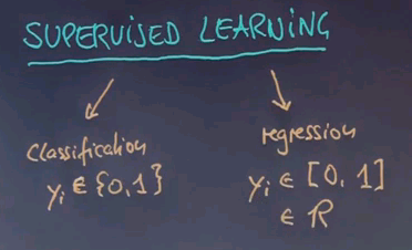
Let me back up a step further, and let's look at supervised learning more generally. Our example so far was one of classification. The characteristic of classification is that the target labels or the target class is discrete. In our case it was actually binary. In many problems, we try to predict a continuous quantity. For example, in the interval 0 to 1 or perhaps a real number. Those machine learning problems are called regression problems. Regression problems are fundamentally different from classification problems.
For example, our Bayes network doesn't afford us an answer to a problem where the target value could be in [0,1]. A regression problem, for example, would be one to predict the weather tomorrow. Temperature is a continuous value. Our Bayes network would not be able to predict the temperature, in only can predict discrete classes. A regression algorithm is able to give us a continuous prediction about the temperature tomorrow. So let's look at the regression next.
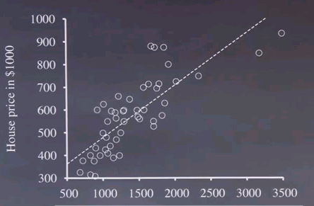
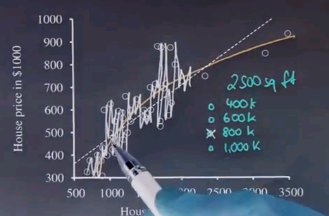
So here's my first quiz for you on regression. This scatter plot shows for Berkeley California for a period of time the data for each house that was sold. Each dot is a sold house. And it graphs the size of the house in square feet to the sale price in thousands of dollars. As you can see, roughly speaking, as the size of the house goes up, so does the sale price.
I wonder, for a house of about 2500 square feet, what is the approximate sales price you would assume based just on the scatter plot data? Is it 400k, 600k, 800k or 1000k?
And my answer is, there seems to be a roughly linear relationship, maybe not quite linear, between the house size and the price. So we look at a linear graph that best describes the data and you get this dashed line over here. And for the dashed line, if you walk up the 2500 square feet, you end up with roughly 800k. So this would have been the best answer.
Linear Regression
Now obviously you can answer this question without understanding anything about regression. But what you find is this is different from classification as before, this is not a binary concept any more of like "expensive" and "cheap", it's really a relationship between two variables. One you care about, the house price, and one that you can observe, which is the house size in square feet. And your goal is to really fit a curve that best explains the data.
Once again we have a case where we can play Occam's Razor, there's clearly a data fit that's non-linear that might be better like this one over here. And when you go to highly non-linear curves you might even be inclined to draw a curve like this:
Now of course the curve I'm drawing right now is likely an overfit and you don't want to postulate that this is the general relationship between the size of a house and the sale price. So even though the black curve might describe the data better the blue curve or the dashed linear curve over here might be better explanations by virtue of Occam's Razor.
So let's look a little bit deeper into what we call regression. As in all regression problems our data will be comprised of input vectors of length n that map to another continuous value. And we might be given a total of m data points.
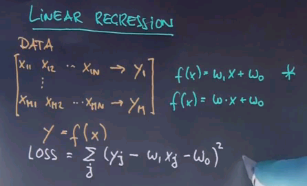
This is familiar from the classification case except this time the ys are continuous. Once again we're looking for a function f that maps our vector x into y. In linear regression the function has a particular form which is f(x) = w1x + w0, in the case that x is one-dimensional, which is n=1. Or in a high-dimensional space we might just write where w is a vector and x is a vector and is the inner product of these two vectors.
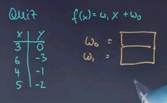
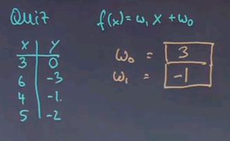
But let's for now just consider the one-dimensional case. In this quiz I'm giving you the linear regression form with two unknown parameters, w1 and w0, and I'm giving you a data set. And this data set happens to be fittable by a linear regression model without any residual error. Without any math, can you look at this and find out for me what the two parameters w0 and w1 are?
This is a surprisingly challenging question. If you look at these numbers from 3 to 6, when we increase x by 3, y decreases by 3, which suggests w1 is -1. Now let's see if this holds. If we increase x by 3, it decreases by 3. If we increase x by 1, we decrease y by 1. If we increase x by 2, we decrease y by 2. So this number seems to be an exact fit. Next we have to get the constant w0 right. For x=3, we get -3 as an expression over here, because we know w1 = -1. So if this has to equal zero in the end, then w0 has to be 3. Let's do a quick check. -3 + 3 is 0. -6 + 3 is -3. And if you plug in the other numbers, you find those are correct. Now this is the case of an exact data set. It gets much more challenging if the data set cannot be fit with a linear function.
More Linear Regression
To define linear regression, we need to understand what we are trying to minimise. The word here is called here a loss function, and the loss function is the amount of residual error we obtain after fitting the linear function as good as possible. The residual error is the sum of all training examples, j of yj, which is the ?? label, minus our prediction, which is w1 xj minus w0 to the square. This is the quadratic error between our target tables and what our best hypothesis can produce.
The minimising of loss is used for linear regression of a any regression problem, and you can write it as follows: Our solution to the regression problem w* is the arg min of the loss over all possible vectors w.
Quadratic Loss
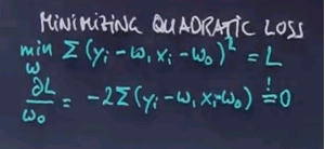
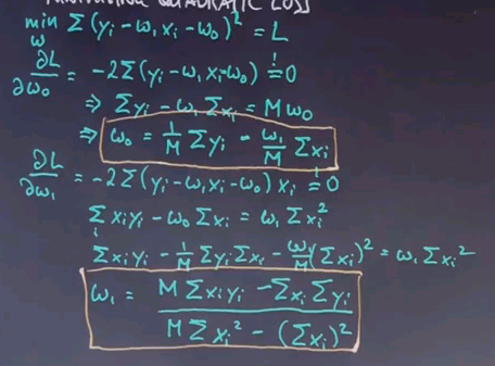
The problem of minimising quadratic loss for linear functions can be solved in closed form. When I do this, I will do this for the one-dimensional case on paper. I will also give you the solution for the case when your input space is multidimensional, which is often called "multivariant regression". We seek to minimise a sum of a quadratic expression where the target labels are subtracted with the output of our linear regression model parameterised by w1 and w0. The summation here is over all training examples, and I leave the index of the summation out if not necessary.
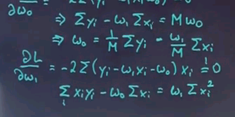
The minimum of this is obtained where the derivative of this function equals zero. So let's call this function L. For the partial derivative with respect to w0, we get this expression over here, which we have to set to zero.
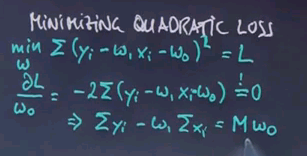
We can easily get rid of the -2 and transform this as follows:
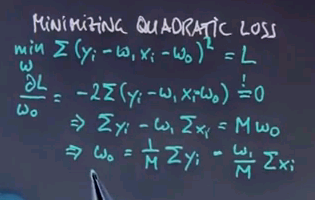
Here M is the number of training examples.
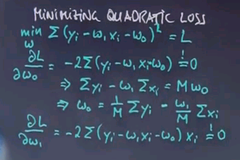
This expression over here gives us w0 as a function of w1, but we don't know w1. Let's do the same trick for w1 and set this to zero as well.
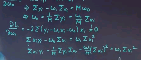
Which gets us the expression over here:
We can now plug in the w0 over here into this expression over here and obtain this expression over here:
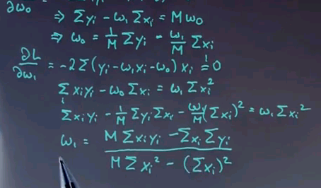
This looks really involved but it's relatively straightforward. With a few steps of further calculation, which I'll spare you for now, we get for w1 the following important formula:
This is the final quotient for w1, where we take the number of training examples times the sum of all x y minus the sum of x times the sum of y divided by this expression over here. Once we've computed w1, we can go back to our original articulation of w0 over here and plug w1 into w0 and obtain w0.
These are the two important formulas you can also find in the textbook:
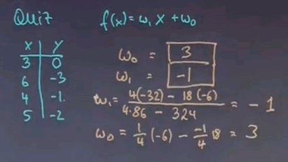
I'd like to go back and use those formulas to calculate these two coefficients over here.
You get 4 times the sum of x and the sum of y, which is -32, minus the product of the sum of x, which is 18, and the sum of y, which is -6, divided by the sum of x squared, which is 86, times 4, minus the sum of x squared, which is 18 times 18, which is 324. If you work this all out, it becomes -1, which is w1.
w0 is now obtained by completing a quarter times sum of all y, which is -6, minus w1 over 4 times the sum of all x. If you plug this all in, you get 3, as over here. Our formula is actually correct.
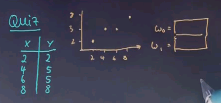
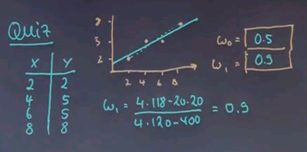
Here is another quiz for linear regression. We have the following data. Here is the data plotted graphically. And I wonder what the best regression is? Give me w0 and w1. Apply the formulas I just gave you.
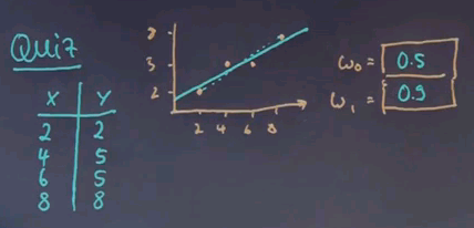
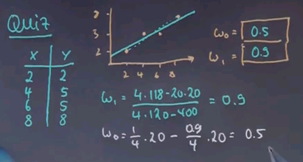
And the answer is w0 = 0.5 and w1 = 0.9. If I were to draw a line, it would go about like this:
It doesn't really hit the two points at the end. So if you were thinking of something like the dashed line, you were wrong. If you draw a curve like this, your quadratic error becomes 2. One over here and one over here. The quadratic error is smaller for the line that goes in between those points. This is easily seen by computing as shown in the previous slide. w1 equals (4 * 118 - 20 * 20) / (4 * 120 - 400) which is 0.9.
This is merely plugging in those numbers into the formulas I gave you. w0 then becomes 1/4 * 20. Now we plug in w1 0.9 / 4 * 20 equals 0.5.
So, this is an example of linear regression, in which case there is a residual error, and the best-fit curve is the one that minimises the total of the residual vertical error in this graph over here.
Problems with Linear Regression
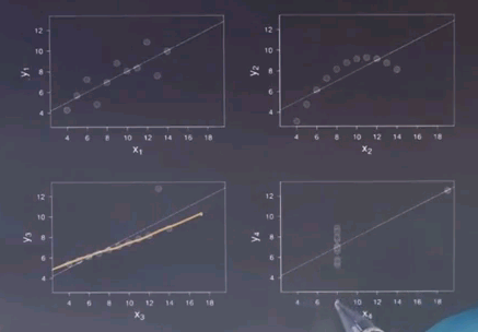
So linear regression works well if the data is approximately linear, but there's many examples where linear regression performs poorly. Here's on where we have a curve that is clearly non-linear. This is an interesting one where we seem to have a linear relationship that is flatter than the linear regression indicates, but there is one outlier. Because if you are minimising quadratic error outliers penalise you over-proportionately. So outliers are particularly bad for linear regression. And here is a case where the data clearly suggests a very different phenomena from linear. We have only two input variables even being used, and this one has a strong frequency and a strong vertical spread. Clearly a linear regression model is a very poor one to explain this data over here.
Another problem with linear regression is that as you go to infinity in the x space, your ys also become infinite. In some problems that isn't a plausible model. For example, if you wish to predict the weather any time into the future, it's implausible to assume the further the prediction goes out the hotter of the cooler it becomes. For such situations there is a model called logistic regression, which uses a slightly more complicated model than linear regression, which goes as follows:
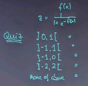
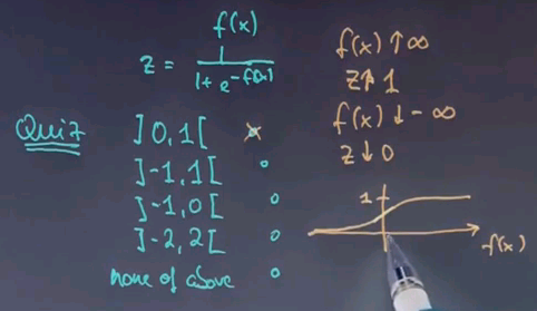
Let f(x) be our linear function, and the output of logistic regression is obtained by the following function: One over one plus exponential of minus f(x).
So here's a quick quiz for you. What is the range in which z might fall given this function over here and the linear function of f(x) over here. Is it 0,1? Is it -1,1? Is it -1,0? -2,2? Or none of the above?
The answer is 0,1. If f(x) grows to positive infinity then z becomes 1. And the reason is that as f(x) becomes very large e to the minus that term approaches zero and one over one equals one. If f(x) goes to minus infinity then z goes to zero. And the reason is if f(x) goes to minus infinity e to the power of infinity becomes very large and one over something very large becomes zero. When we plot the logistic function it looks like this:
So it's approximately linear around f(x) = 0, but it levels off to zero and one as we go to the extremes.
Linear Regression and Complexity Control
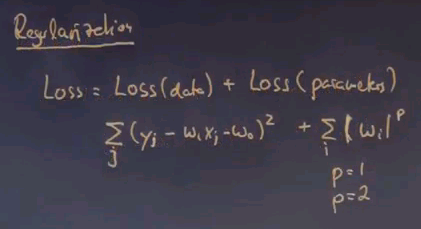
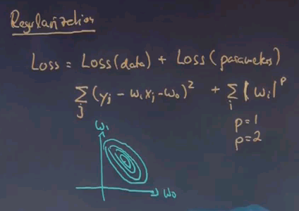
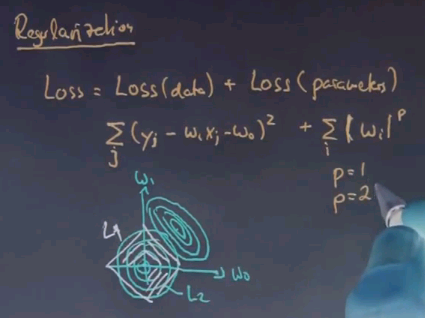
Another problem with linear regression has to do with the regularisation, or complexity control. Just like before, we sometimes with to have a less complex model. So in regularisation, the loss function is usually the sum of the loss of a data function and a complexity control term, which is often called loss over the parameters. The loss over data is typically quadratic loss, as we discussed before. And the loss over parameters might just be a function that penalises the parameters to become large, up to some known P, where P is usually either 1 or 2.
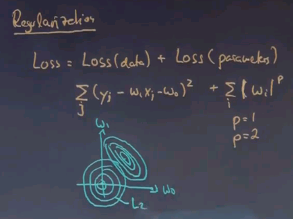
If you draw this graphically, in a parameter space comprising two parameters, your quadratic term for minimising the data error might look like this, where the minimum sits over here.
Your term for regularisation might pull these parameters toward zero. It pulls it toward zero, along the circle if you use quadratic error,
and it does it in a diamond shaped way for L1 regularisation,
either one works well.
L1 has the advantage in that parameters tend to get really sparse. If you look at this diagram there is a tradeoff between w0 and w1 in the L1 case that allows one of them to be driven to zero. In the L2 case parameters tend not to be as sparse, so L1 is often preferred.
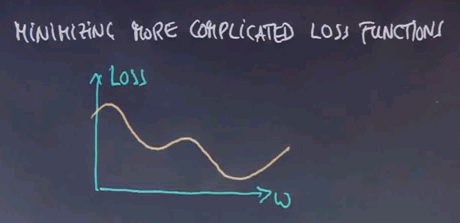
Minimizing Complicated Loss Functions
This all raises the question, how to minimise more complicated loss functions than the one we discussed so far. Are there closed-form solutions of the type we found for linear regression? Or do we have to resort to iterative methods?
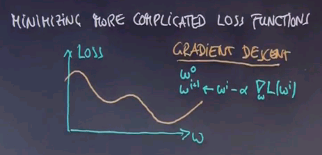
The general answer is, unfortunately, we have to resort to iterative methods. Even though there are special cases in which closed-form solutions may exist, in general, our loss functions now become complicated enough that all we can do is iterate.
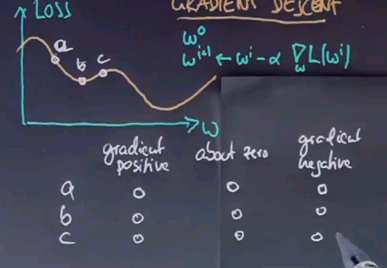
Here is a prototypical loss function, and the method for iteration will be called gradient descent. In gradient descent, you start with an initial guess, w0, where 0 is your iteration number, and then you update it iteratively. Your i+1 parameter guess will be obtained by taking your i-th guess and subtracting from it the gradient of your loss function and that guess, multiplied by a small learning weight alpha, where alpha is often as small as 0.01.
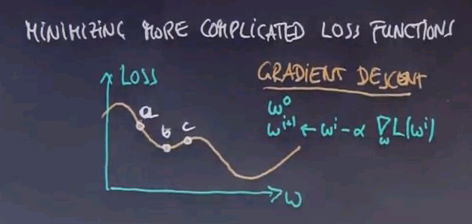
I have a couple of questions for you. Consider the following three points:
We call them a, b, c. I wish to know, for points a, b, and c, is the graident at this point positive, about zero, or negative? For each of those, check exactly one of those cases.
In case A, the gradient is negative. If you move to the right in the x space, then your loss decreases. In B, it's about zero; and in C, it's pointing up, it's positive. So if you apply the rule over here, if you were to start at A as your w0, then your gradient is negative. Therefore, you would add something to the value of w. You move to the right, and your loss has decreased. You do this until you find yourself with what's called a local minimum, where B resides. In this instance over here, gradient descent starting at A would not get you to the global minimum, which sits over here, because there's a bump in between. Gradient methods are known to be subject to local minima.
Question
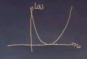
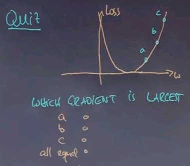
I have another gradient quiz. Consider the following quadratic error function.
We are considering the gradient in three different places, a, b, and c. And I ask you which gradient is the largest, a, b, or c, or are they all equal? In which case you would want to check the last box over here.
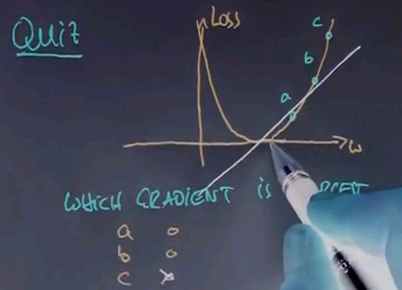
And the answer is c. The derivative of a quadratic function is a linear function, which will look about like this:
And as we go outside, our gradient becomes larger and larger. This over here is much steeper than this curve over here.
Question
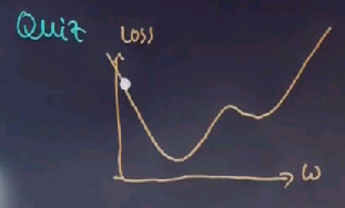
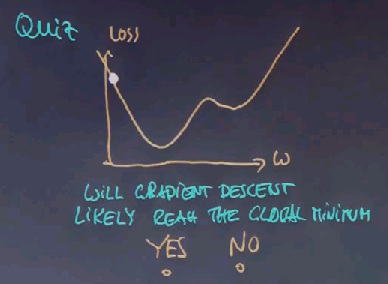
Here is a final gradient descent quiz. Suppose we have a loss function like this, and our gradient descent starts over here:
Will it likely reach the global minimum? Yes or no. Please check on of those boxes.
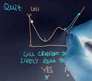
And the answer is yes, although, technically speaking, to reach the absolute global minimum we need the learning rate to become smaller and smaller over time. If they stay constant there is a chance this thing might bounce around between 2 points at the end and never reach the global minimum. But assuming that we implement gradient descent correctly, we will finally reach the global minimum. Now that's not the case if you start over here, where we can get stuck over here,
and settle for the minimum over here, which is a local minimum and not the best solution to our optimisation problem. So one of the important points to take away from this is gradient descent is fairly universally applicable to more complicated problems -- problems that don't have a closed-form solution. But you have to check whether there is many local minima, and if so you have to worry about this. Any optimisation book can tell you tricks how to overcome this. I won't go into any more depth here in this class.
Gradient Descent Implementation
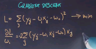
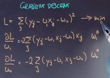
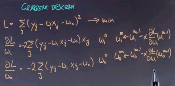
It's interesting to see how to minimise a loss function using gradient descent. In our linear case, we have L equals sum over the correct labels minus our linear function to the square, which we seek to minimise.
Now we already know that this is a closed-form solution, but just for the fun of it, let's look at gradient descent. The gradient of L with respect to w1 is minus 2, sum of all j, of the difference as before but without the square time xj.
The gradient with respect to w0 is very similar.
So in gradient descent we start with w10 and w00, where the upper 0 corresponds to the iteration index of gradient descent. And then we iterate. In the m-th iteration we get our new estimate by using the old estimate minus a learning rate of this gradient over here taking the position of the old estimate w1 m-1. Similarly, for w0 we get this expression over here.
And these expressions look nasty, but what it really means is we subtract an expression like this every time we do gradient descent from w1 and an expression like this every time we do gradient descent from w0, which is easy to implement, and that implements gradient descent.
Perceptron and SVMs
Now, there are many different ways to apply linear functions in machine learning. We so far have studied linear functions for regression, but linear functions are also used for classification, and specifically for an algorithm called the perceptron algorithm. This algorithm happens to be a very early model of a neuron, as in the neurons we have in our brains, and it was invented in the 1940s.
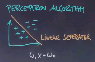
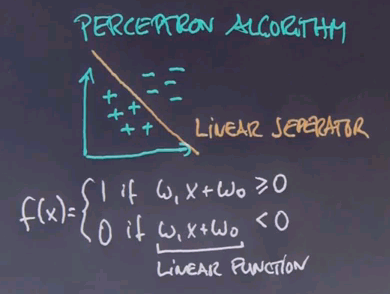
Suppose we are given a data set of positive samples and negative samples. A linear separator is a linear equation that separates positive from negative examples. Obviously not all data sets posses a linear separator, but some do. And for those we can define the algorithm of the perceptron and it actually converges.
To define a linear separator, let's start with our linear equation as before -- w1x + w0.
In cases where x is higher dimensional this might actually be a vector -- never mind. If this is larger or equal to zero, then we call our classification 1. Otherwise we call it 0. So here's our linear separation classification function, where this is our common linear function.
Now, as I said, perceptron only converges if the data is linearly separable, and then it converges to a linear separation of the data, which is quite amazing. Perceptron is an iterative algorithm that is not dissimilar from gradient descent. In fact, the update rule echoes that of gradient descent, and here's how it goes.
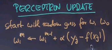
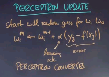
We start with a random guess for w1 and w0, which may correspond to a random separation line, but usually is inaccurate. Then the m-th weight i is obtained by using the old weight plus some learning rate alpha times the difference between the desired target label and the target label produced by our function at the point m-1.
Now, this is an online learning rule, which is we don't process all the data in batch. We process one data at a time, and we might go through the data many many times -- hence the j over here -- but every time we do this we apply this rule over here.
What this rule gives us is a method to adapt our weights in proportion to the error. If the prediction of our function f equals our target label, then the error is zero, and no update occurs. If there is a difference however, we update in a way so as to minimise the error. Alpha is a small learning rate.
Once again, perceptron converges to a correct linear separator if such a linear separator exists.
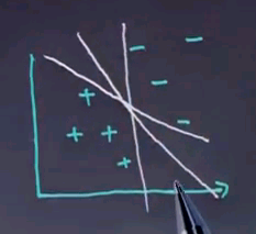
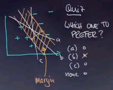
Now the case of linear separation has recently received a lot of attention in machine learning. If you look at the picture over here, you'll find there are many different linear separators.
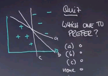
One of the questions that has recently been researched extensively is which one to prefer. Is it a, b, or c? And even though you probably have never seen this literature, I will just ask your intuition in this following quiz. Which linear separator would you prefer if you look at these three different linear separators -- a, b, c, or none of them?
And intuitively I would argue it's B, and the reason why is C comes really close to examples. So if these examples are noisy, it's quite likely that by being so close to these examples that future examples cross the line. Similarly A comes close to examples. B is the one that stays really far away from any example. So there's this entire region over here where there's no example anywhere near B. This region is often called the margin.
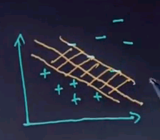
The margin of the linear separator is the distance of the separator to the closest training example. The margin is a really important concept in machine learning. There's an entire class of maximum margin learning algorithms, and the two most popular are support vector machines and boosting. If you are familiar with machine learning, you've come across these terms. These are very frequently used these days in actual discrimination learning tasks. I will not go into any details because it would go way beyond the scope of this introduction to artificial intelligence class, but let's see a few abstract words specifically about support vector machines, or SVMs.
As I said before a support vector machine derives a linear separator, and it takes the one that actually maximises the margin as shown over here.
By doing so it attains additional robustness over perceptron which only picks a linear separator without consideration of the margin.
Now the problem of finding the margin maximising linear separator can be solved by a quadratic program which is an iterative method for finding the best linear separator that maximises the margin. One of the nice things that support vector machines do in practice is they use linear techniques to solve nonlinear separation problems, and I'm just going to give you a glimpse of what's happening without going into any detail.
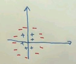
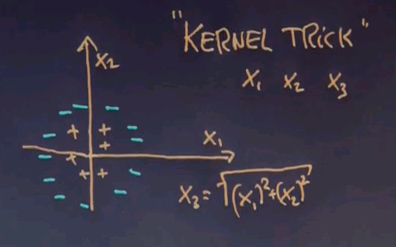
Suppose the data looks as follows:
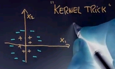
We have a positive class which is near the origin of a coordinate system and a negative class that surrounds the positive class. Clearly these two classes are not linearly separable because there's no line I can draw that separates the negative examples from the positive examples. An idea that underlies SVMs, that will ultimately be known as the kernel trick, is to augment the feature set by new features.
Suppose this is x1 and this is x2,
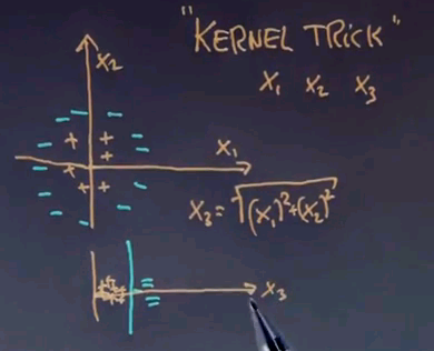
and normally x1 and x2 will be the input features. In this example you might derive a third one. Let me pick a third one. Suppose x3 equals the square root of x12 + x22.
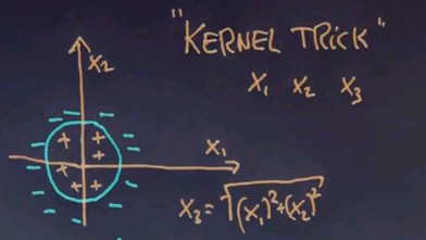
In other words x3 is the distance of any data point from the centre of the coordinate system. Then things do become linearly separable. Plotted just along the third dimension all the positive examples end up to be close to the origin, and all the negative examples are further away and the line that is orthogonal to the third input feature solves the separation problem.
Mapped back into the space over here it's actually a circle, which is a set of all values of x3 that are equidistant to the centre of the circle at the origin.
Now this trick could be done in any linear learning algorithm, and it's really an amazing trick. You can take any nonlinear problem, add features of this type or any other type, and use linear techniques and get better solutions. This is a very deep machine learning insight that you can extend your feature space in this way, and there's numerous papers written about this.
In SVMs, the extension of the feature space is mathematically done by what's called a kernel. I can't really tell you what it is in this class, but it makes it possible to derive very large new feature spaces including infinitely dimensional new feature spaces. These methods are very powerful. It turns out you never really compute all those features. They are implicitly represented by so called kernels, and if you care about this, I recommend you dive deeper into the literature of support vector machines. This is meant to just give you an overview of the essence of what support vector machines are all about.
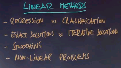
So in summary, in linear methods, we learned about using them for regression and also classification. We learned about exact solutions versus iterative solutions. We talked about smoothing, and we even talked about using linear methods for nonlinear problems.
So we covered quite a bit of ground. This is a really significant cross section of machine learning.
k Nearest Neighbours
As the final method in this unit, I'd like now to talk about k-nearest neighbours. And the distinguishing factor of k-nearest neighbours is that it is a nonparametric machine learning method. So far we've talked about parametric methods. Parametric methods have parameters, like probabilities or weights, and the number of parameters is constant. Or put differently, the number of parameters is independent of the training set size. So for example in the Naive Bayes, if we bring up more data, the number of conditional probabilities will stay the same. Well, that wasn't technically always the case. Our vocabulary might increase and as such the number of parameters. But for any fixed dictionary, the number of parameters are truly independent of the training set size. The same was true, for example, in our regression cases where the number of regression weights is independent of the number of data points. Now this is very different from non-parametric where the number of parameters can grow. In fact it can grow a lot over time. Those techniques are called non-parametric.
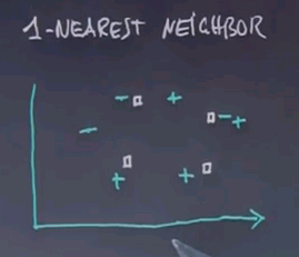
Nearest neighbour is so straightforward. I'd really like to introduce you using a quiz. So here's my quiz. Suppose we have a number of data points. I want you for 1-nearest neighbour to check those squared areas that you believe will carry a positive label. And I will give you the label of the existing data points. So please check any of those boxes that you believe are now 1-nearest neighbour that carry a positive label. And the algorithm, of course, searches for the nearest point in this Euclidean space and just copies its label.
k NN Definition
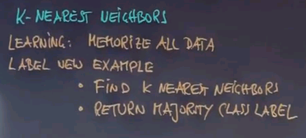
The algorithm is really blatantly simple. In the learning step you simply memorise all data. If a new example comes along with the input value you know, but which you wish to classify, you do the following. You first find the k-nearest neighbours. And then you return the majority class label as your final class label for the new example.
Simple, isn't it?
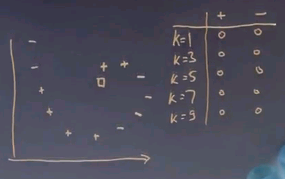
So here's a somewhat contrived situation of the data point we wish to classify where the label data lies on the spiral of increasing diameter as it goes outwards. Please answer for me in this quiz what class label you'd assign for k = 1, k = 3, 5, 7, and all the way to 9.
And this is easily answered. The nearest neighbour is this point over here, so for 1 we say plus. For 3 neighbours, we get 2 positive, 1 negative. It's still plus. For 5 neighbours -- 1, 2, 3, 4, 5 -- we get 3 negative, 2 positive. It's a minus. For 7, we get 3 positive but still 4 negative, so it's negative. And for 9, the positives outweigh the negative, so you get a plus. Obviously, as you can see, a k increases, more and more data points are being consulted. So when k finally becomes 9 all those data points are in and make a much smoother result.
k as Smoothing Parameter
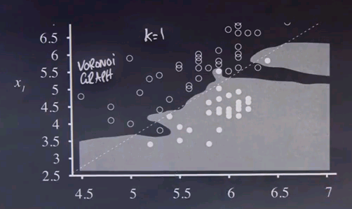
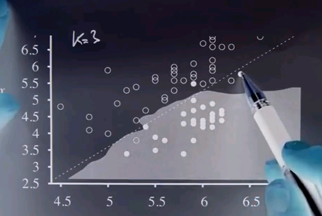
Just as in the Laplacian smoothing example before, the value of k is a smoothing parameter. It makes the function less scattered. Here's an example of k=1 for a 2-class nearest neighbour problem. You can see the separation boundary is what's called a Voroni diagram, between the positive and negative class, and in cases where there is noise between these class boundaries, you'll find really funny, complex boundaries as indicated over here.
Particularly interesting is this guy over here where this class of the circle over here protrudes way into the otherwise solid class. Now, as you go to k=3, you get this graph over here, which is smoother.
So if you are over here, your two nearest neighbours are of this type over there, and you get a uniform class over here. In this region over here, you get uniform classes as solid classes as shown over here. The more you drive up k, the more clean this decision boundary becomes, but the more outliers are actually misclassified as well.
So if I go back to my k-nearest neighbour method, we just learned that k is a regulariser. It controls the complexity of the k-nearest neighbour algorithm, and the larger k is, the smoother the output. We can, once again, use cross-validation to find the optimal k because there is an inherent trade off between the complexity of what we want to fit and the goodness of the fit.
Problems with kNN
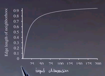
What are the problems of kNN? Well, I would argue that there's two. One is very large data sets, and one is very large feature spaces. Now the first one results in lengthy searches when you try to find the k's nearest neighbours. Now, fortunately there are methods to search efficiently. Often you represent your data not by a linear list, in which case the search would be linear in the number of data points, but by a tree, where the search becomes logarithmic. The method of choice is called kdd trees where there's many other ways to represent data points as trees. Now very large feature spaces cause more of a problem. It turns out computing nearest neighbours, as the feature space for the input vector increases, it becomes increasingly difficult, and the tree methods become increasingly brittle. And the reason is shown in the following graph:
If you graph your input dimension to the average edge length of your neighbourhood you'll find that for randomly chosen points very quickly all points are really far away. The edge length of one is obtained if your query point is unit one away from the nearest neighbour. If you have one hundred dimensions, that is almost certain. Why is that? Well, in one hundred dimensions, there ought to be one where just by chance you're far away. The number of points you need to get something close grows exponentially with the number of dimensions. So, for any fixed data set size you will find yourself in a situation where all your neighbours are far away. Nearest neighbour works really well for small input spaces like three or four dimensions. It works very poorly if your input space is twenty, twenty-five, or maybe one hundred dimensions. So don't trust nearest neighbour to do a good job if your input and measure spaces are high.
Congratulations
So congratulations. You've just learned a lot about machine learning. We focused on supervised machine learning which deals with situations where you have input vectors and given output labels and your goal is to predict the output label from an input vector. And we looked into parametric models, like Naive Bayes, and non-parametric models. We talked about classification where the output is discrete versus regression where the output is continuous and we looked at samples of techniques for each of these situations.
Now obviously we just scratched the surface of machine learning. There's books written about it and courses taught about it. Machine learning is a super fascinating topic. It's the one within the artificial intelligence I love the most. It's really great about the real world as we gain more data like the world wide web or medical data sets or financial data sets, machine learning is poised to become more and more important. I hope that the things you learned in this class so far really excite you and entice you to apply machine learning to problems that you face in your professional life.
