AI class unit 4
These are my notes for unit 4 of the AI class.
Probabilistic Inference
Overview and Example
Welcome back. In the previous unit, we went over the basics of probability theory and saw how a Bayes network could concisely represent a joint probability distribution, including the representation of independence between the variables. In this unit, we will see how to do probabilistic inference. That is, how to answer probability questions using Bayes nets.
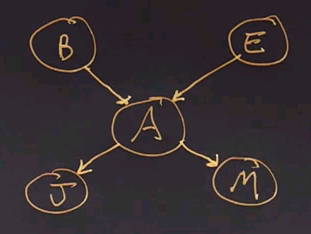
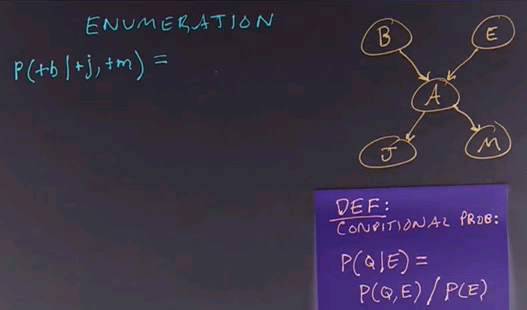
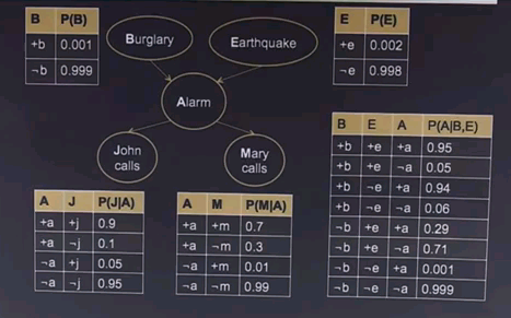
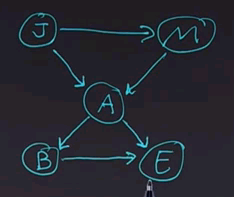
Let's put up a simple Bayes net. We'll use the familiar example of the earthquake where we can have a burglary (B) or an earthquake (E) setting off an alarm (A), and if the alarm goes off, either John (J) or Mary (M) might call.
Now, what kinds of questions can we ask to do inference about? The simplest type of question is the same question we ask with an ordinary subroutine or function in a programming language. Namely, given some inputs, what are the outputs? So, in this case, we could say given the inputs of B and E, what are the outputs J and M?
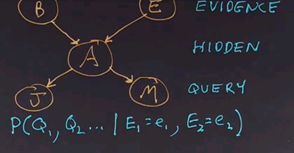
Rather than call them input and output variables, in probabilistic inference, we'll call them evidence and query variables. That is, the variables that we know the values of are the evidence, and the ones that we want to find out the values of are the query variables. Anything that is neither evidence nor query is known as a hidden variable. That is, we won't tell you what its value is. We won't figure out what its value is and report it, but we'll have to compute with it internally.
And now furthermore, in probabilistic inference, the output is not a single number for each of the query variables, but rather it's a probability distribution. So, the answer is going to be a complete, joint probability distribution over the query variables. We call this the posterior distribution, given the evidence, and we can write it like this:
It's the probability distribution of one or more query variables given the values of the evidence variables. And there can be zero or more evidence variables, and each of them are given an exact value. And that's the computation we want to come up with.
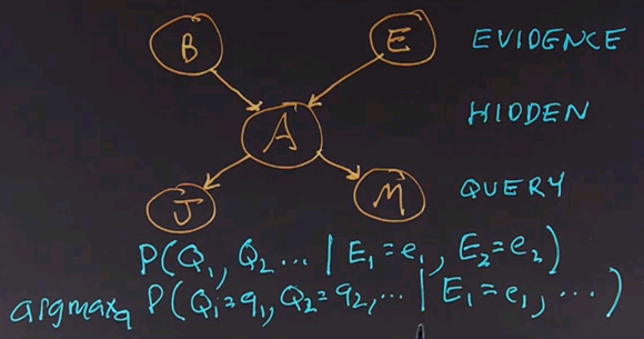
There's another question we can ask. Which is the most likely explanation? That is, out of all the possible values for all the query variables, which combination of values has the highest probability?
We write the formula like this:
asking which Q values are maximal given the evidence values. Now, in an ordinary programming language, each function goes only one way. It has input variables, does some computation, and comes up with a result variable or result variables. One great thing about Bayes nets is that we're not restricted to going only in one direction. We could go in the causal direction, giving as evidence the root nodes of the tree and asking as query values the nodes at the bottom. Or, we could reverse that causal flow. For example, we could have J and M be the evidence variables and B and E be the query variables, or we could have any other combination. For example, we could have M be the evidence variable and J and B be the query variables.
Here's a question for you. Imagine the situation where Mary has called to report that the alarm is going off, and we want to know whether or not there has been a burglary. For each of the nodes, click on the circle to tell us if the node is an evidence node, a hidden node, or a query node.
The answer is that Mary calling is the evidence node. The burglary is the query node, and all the others are hidden variables in this case.
Enumeration
Now we're going to talk about how to do inference on Bayes nets. We'll start with our familiar network, and we'll talk about a method called enumeration, which goes through all the possibilities, adds them up, and comes up with an answer.
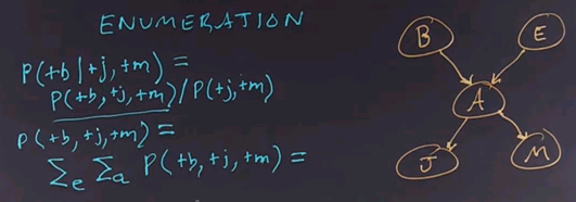
So, what we do is start by stating the problem. We're going to ask the question of what is the probability that the burglar alarm occurred given that John called and Mary called? We'll use the definition of conditional probability to answer this.
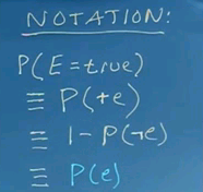
So, this query is equal to the joint probability distribution of all 3 variables divided by the conditionalized variables. Now, note that I'm using a notation here where instead of writing out the probability of some variable equals true, I'm just using the notation plus and then the variable name in lower case, and if I wanted the negation, I would use the negation sign. Notice there's a different notation where instead of writing out the plus and negation signs, we just use the variable name itself, P(e), to indicate E is true.
That notation works well, but it can get confusing between does P(e) mean E is true, or does it mean E is a variable? And so we're going to stick to the notation where we explicitly have the pluses and negation signs.
To do inference by enumeration, we first take a conditional probability and rewrite it as unconditional probabilities. Now we enumerate all the atomic probabilities can calculate the sum of products. Let's look at just the complex term on the numerator first. The procedure for figuring out the denominator would be similar, and we'll skip that.
So, the probability of these three terms together can be determined by enumerating all possible values of the hidden variables. In this case there are 2, E and A. So we'll sum over those variables for all values of E and for all values of A. In this case they're boolean, so there's only two values of each. We ask what's the probability of this unconditional term? And that we get by summing out over all possibilities, E and A being true or false.
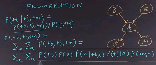
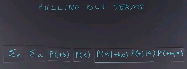
Now, to get the values of these atomic events, we'll have to rewrite this equation in a form that corresponds to the conditional probability tables that we have associated with the Bayes net. So, we'll take this whole expression and rewrite it. It's still a sum over the hidden variables E and A, but now I'll rewrite this expression in terms of the parents of each of the nodes in the network. So, that gives us the product of these five terms, which we then have to sum over all values of E and A.
If we call this product f(e,a), then the whole answer is the sum of F for all values of E and A, so it's the sum of four terms where each of the terms is a product of five numbers.
Where do we get the numbers to fill in this equation?
From the conditional probability tables from our model, so let's put the equation back up, and we'll ask you for the case where both E and A are positive to look up in the conditional probability tables and fill in the numbers for each of these five terms, and then multiply them together and fill in the product.
We get the answer by reading numbers off the conditional probability tables, so the probability of B being positive is 0.001. Of E being positive, because we're dealing with the positive case now for the variable e, is 0.002. The probability of A being positive, because we're dealing with that case, given that B is positive and the case for an E is positive, that we can read off here as 0.95. The probability that J is positive given that A is positive is 0.9. And finally, the probability that M is positive given that A is positive we read off here as 0.7. We multiply all those together, it's going to be a small number because we've got the 0.001 and the 0.002 here. Can't quite fit it in the box, but it works out to 0.000001197. That seems like a really small number, but remember, we have to normalize by the P(+j,+m) term, and this is only one of the four possibilities. We have to enumerate over all four possibilities for E and A, and in the end, it works out that the probability of the burglar alarm being true given that John and Mary calls, is 0.284.
And we get that number because, intuitively, it seems that the alarm is fairly reliable, John and Mary calling are very reliable, but the prior probability of burglary is low. And those two terms combine together to give us the 0.284 value when we sum up each of the four terms of these products.
Speeding Up Enumeration
We've seen how to do enumeration to solve the inference problem on belief networks. For a simple network like the alarm network, that's all we need to know. There's only five variables, so even if all five of them were hidden, there would only be 32 rows in the table to sum up. From a theoretical point of view, we're done. But from a practical point of view, other networks could give us trouble. Consider this network, which is one for determining insurance for car owners. There are 27 difference variables. If each of the variables were boolean, that would give us over 100 million rows to rum out. But in fact, some of the variables are non-boolean, they have multiple values, and it turns out that representing this entire network and doing enumeration we'd have to sum over a quadrillion rows. That's just not practical, so we're going to have to come up with methods that are faster than enumerating everything.
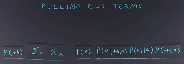
The first technique we can use to get a speed-up in doing inference on Bayes nets is to pull out terms from the enumeration.
For example, here the probability of B is going to be the same for all values of E and A. So we can take that term and move it out of the summation, and now we have a little bit less work to do.
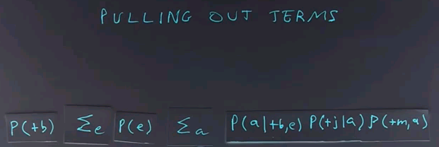
We can multiply by that term once rather than having it in each row of the table. We can also more this term, P(e), to the left of the summation over a, because it doesn't depend on a.
By doing this, we're doing less work. The inner loop of the summation now has only three terms rather than five terms. So we've reduced the cost of doing each row of the table. But we still have the same number of rows in the table, so we're gonna have to do better than that.
The next technique for efficient inference is to maximise the independence of variables. The structure of a Bayes net determines how efficient it is to do inference on it. For example, a network that's a linear string of variables, X1 through Xn, can have inference done in time proportional to the number n,
whereas a network that's a complete network where every node points to every other node and so on could take time 2n if all n variables are boolean variables.
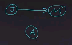
In the alarm network we saw previously, we took care to make sure that we had all the independence relations represented in the structure of the network. But if we put the nodes together in a different order, we would end up with a different structure. Let's start by ordering the node "John calls" first. And then adding the node "Mary calls". The question is, given just these two nodes and looking at the node for "Mary calls", is that node dependent or independent of the node for "John calls"?
The answer is that the node for "Mary calls" in this network is dependent on "John calls". In the previous network, they were independent given that we know that the alarm had occurred. But here we don't know that the alarm had occurred, and so the nodes are dependent because having information about one will affect the information about the other.
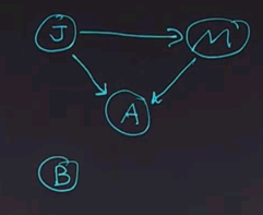
Now we'll continue and we'll add the node A for alarm to the network. And what I want you to do is click on all the other variables that A is dependent on in this network.
The answer is that alarm is dependent on both John and Mary. And so we can draw both nodes in, both arrows in. Intuitively that makes sense because if John calls, then it's more likely that the alarm has occurred, likely as if Mary calls, and if both called, it's really likely. So you can figure out the answer by intuitive reasoning, or you can figure it out by going to the conditional probability tables and seeing according to the definition of conditional probability whether the numbers work out.
Now we'll continue and we'll add the node B for burglary, and ask again, click on all the variables that B is dependent on.
The answer is that B is dependent only on A. In other words, B is independent of J and M given A.
And finally, we'll add the last node, E, and ask you to click on all the nodes that E is dependent on.
And the answer is that E is dependent on A. That much is fairly obvious. But it's also dependent on B. Now, why is that? E is dependent on A because if the earthquake did occur, then it's more likely that the alarm would go off. On the other hand, E is also dependent on B because if a burglary occurred, then that would explain why the alarm is going off, and it would mean that the earthquake is less likely.
Causal Direction
The moral is that Bayes nets tend to be the most compact and thus the easier to do inference on when they're written in the causal direction -- that is, when the networks flow from causes to effects.
Variable Elimination
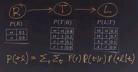
Let's return to this equation, which we use to show how to do inference by enumeration.
In this equation, we join up the whole joint distribution before we sum out over the hidden variables. That's slow, because we end up repeating a lot of work. Now we're going to show a new technique called variable elimination, which in many networks operates much faster. It's still a difficult computation, an NP-hard computation, to do inference over Bayes nets in general. Variable elimination works faster than inference by enumeration in most practical cases. It requires an algebra for manipulating factors, which are just names for multidimensional arrays that come out of these probabilistic terms.
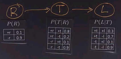
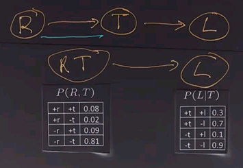
We'll use another example to show how variable elimination works. We'll start off with a network that has three boolean variables. R indicates whether or not it's raining. T indicates whether or not there's traffic, and T is dependent on whether it's raining. And finally, L indicates whether or not I'll be late for my next appointment, and that depends on whether or not there's traffic.
Now we'll put up the conditional probability tables for each of these three variables.
And then we can use inference to figure out the answer to questions like "Am I going to be late?" And we know by definition that we could do that through enumeration by going through all the possible values for R and T and summing up the product of these three nodes.
Now, in a simple network like this, straight enumeration would work fine, but in a more complex network, what variable elimination does is give us a way to combine together parts of the network into smaller parts and then enumerate over those smaller parts and then continue combining. So, we start with a big network. We eliminate some of the variables. We compute by marginalising out, and then we have a smaller network to deal with, and we'll show you how those two steps work.
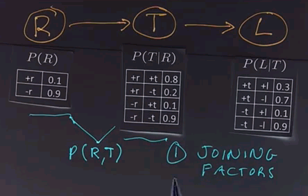
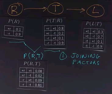
The first operation in variable elimination is called joining factors. A factor, again, is one of these tables. It's a multidimensional matrix, and what we do is choose two of the factors, two or more of the factors. In this case we'll choose these two, and we'll combine them together to form a new factor which represents the joint probability of all the variables in that factor. In this case, R and T.
Now we'll draw out that table. In each case we just look up in the corresponding table, figure out the numbers, and multiply them together.
For example, in this row we have +r and +t, so the +r is 0.1, and the entry for +r and +t is 0.8, so multiply them together and you get 0.08. Go all the way down. For example, in the last row we have a -r and a -t. -r is 0.9. The entry for -r and -t is also 0.9. Multiply those together and you get 0.81.
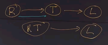
So, what have we done? We used the operation of joining factors on these two factors (R and T), giving us a new factor which is part of the existing network.
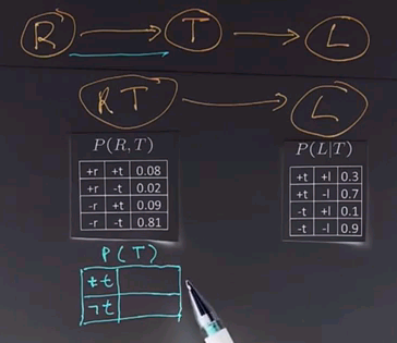
Now we want to apply a second operation called elimination, also called summing out or marginalisation, to take this table and reduce it. Right now the tables we have look like this:
We could sum out or marginalise over the variables R to give us a table that just operates on T. So the question is to fill in this table for P(T) --
there will be two entires in this table, the +t entry formed by summing out all the entries here for all values of r for which t is positive; and the -t entry, formed the same way, by looking in this table and summing up all the rows over all values of r where t is negative. Put your answer in the boxes.
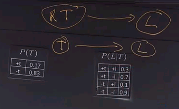
The answer is that for +t we look up the two possible values for r, and we get 0.08 and 0.09. Sum those up, to get 0.17. Then we look at the two possible values of R for -t, and we get 0.02 and 0.81. Add those up, and we get 0.83.
So, we took our network with RT and L. We summed out over R. That gives us a new network with T and L with these conditional probability tables.
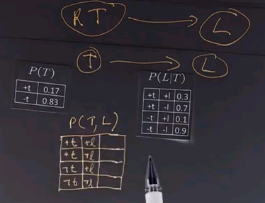
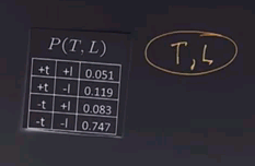
And now we want to do a join over T and L and give us a new table with the joint probability of P(T,L). And that table is going to look like this.
The answer, again, for joining variables is determined by pointwise multiplication, so we have 0.17 times 0.3 is 0.051, +t and -l, 0.17 times 0.7 is 0.119. Then we go to the minuses. 0.83 times 0.1 is 0.083. And finally, 0.83 times 0.9 is 0.747.
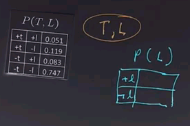
Now we're down to a network with a single node, T, L, with this joint probability table, and the only operation we have left to do is to sum out to give us a node with just L in it.
So, the question is to compute P(L) for both values of L, +l and -l.
Note: in the video an incorrect answer 0.886 is given, the answer should be 0.866.
The answer is that the +l values, 0.051 plus 0.083 equals 0.134. And the negative values, 0.119 plus 0.747 equals 0.866.
So, that's how variable elimination works. It's a continued process of joining together factors to form a larger factor and then eliminating variables by summing out. If we make a good choice of the order in which we apply these operations, then variable elimination can be much more efficient than just doing the whole enumeration.
Approximate Inference
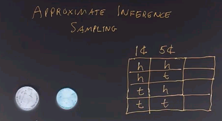
Now I want to talk about approximate inference by means of sampling. What do I mean by that? Say we want to deal with a joint probability distribution, say the distribution of heads and tails over these two coins. We can build a table and then start counting by sampling.
Here we have our first sample. We flip the coins and the one-cent piece came up heads, and the five cent piece came up tails, so we would mark down one count. Then we'd toss them again. This time the five cents is heads, and the one cent is tails, so we put down a count there, and we'd repeat that process and keep repeating it until we got enough counts that we could estimate the joint probability distribution by looking at the counts.
Now, if we do a small number of samples, the counts might not be very accurate. There may be some random variation that causes them not to converge to their true values, but as we add more counts, the counts -- as we add more samples, the counts we get will come closer to the true distribution. Thus, sampling has an advantage over inference in that we know a procedure for coming up with at least an approximate value for the joint probability distribution, as opposed to exact inference, where the computation may be very complex.
There's another advantage to sampling, which is if we don't know what the conditional probability tables are, as we did in our other models, if we don't know these numeric values, but we can simulate the process, we can still proceed with sampling, whereas we couldn't with exact inference.
Sampling Example
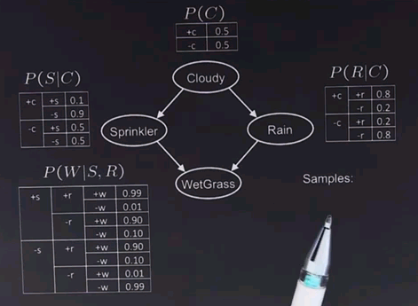
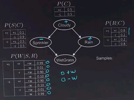
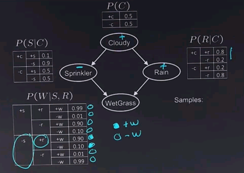
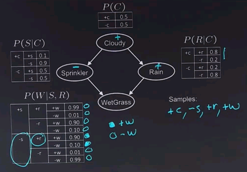
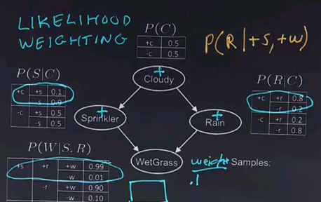
Here's a new network that we'll use to investigate how sampling can be used to do inference. In this network, we have four variables. They're all boolean. Cloudy tells us if it's cloudy or not outside, and that can have an effect on whether the sprinklers are turned on, and whether it's raining. And those two variables in turn have an effect on whether the grass gets wet. Now, to do inference over this network using sampling, we start off with a variable where all the parents are defined. In this case, there's only one such variable, Cloudy. And it's conditional probability table tells us that the probability if 50% for Cloudy, and 50% for not Cloudy, and so we sample from that. We generate a random number, and let's say it comes up with positive for Cloudy. Now that variable is defined, we can choose another variable. In this case let's choose Sprinkler, and we look at the rows in the table for which Cloudy, the parent, is positive, and we see we should sample with probability 10% to +s and 90% to -s. And so let's say we do that sampling with a random number generator, and it comes up negative for Sprinkler. Now let's jump over here. Look at the Rain variable. Again, the parent, Cloudy, is positive, so we're looking at this part of the table. We get a 0.8 probability for Rain being positive, and a 0.2 probability for Rain being negative. Let's say we sample that randomly, and it comes up Rain is positive. And now we're ready to sample the final variable, and what I want you to do is tell me which of the rows of this table should we be considering and tell me what's more likely. Is it more likely that we have a +w or a -w?
The answer to the question is that we look at the parents. We find that the Sprinkler variable is negative, so we're looking at the bottom of the table. And the Rain variable is positive, so we're looking at this part. So, it would be these two rows that we would consider, and thus we'd find there's a 0.9 probability for w, the grass being wet, and only 0.1 for it being negative, so the positive is more likely.
And once we've done that, then we generated a complete sample, and we can write down the sample here. We had +c, -s, +r. And assuming we got a probability of 0.9 came out in favour of the +w, that would be the end of the sample.
Then we could throw all this information out and start over again by having another 50/50 choice for cloudy and then working our way through the network.
Approximate Inference 2
Now, the probability of sampling a particular variable, choosing a +w or a -w, depends on the values of the parents. But those are chosen according to the conditional probability tables, so in the limit, the count of each sampled variable will approach the true probability. That is, with an infinite number of samples, this procedure computes the true joint probability distribution. We say that the sampling method is consistent.
We can use this kind of sampling to compute the complete joint probability distribution, or we can use it to compute a value for an individual variable. But what if we wanted to compute a conditional probability? Say we wanted to compute the probability of wet grass given that it's not cloudy. To do that, the sample that we generated here wouldn't be helpful at all because it has to do with being cloudy, not with being not cloudy. So we would cross this sample off the list. We would say that we reject the sample, and this technique is called rejection sampling. We go through ignoring any samples that don't match the conditional probabilities that we're interested in and keeping samples that do, say the sample -c, +s, +r, -w. We would just continue going through generating samples, crossing off the ones that don't match, keeping the ones that do. And this procedure would also be consistent. We call this procedure rejection sampling.
Rejection Sampling
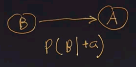
But there's a problem with rejection sampling. If the evidence is unlikely, you end up rejecting a lot of the samples. Let's go back to the alarm network where we had variables for burglary and for an alarm and say we're interested in computing the probability of a burglary, given that the alarm goes off.
The problem is that burglaries are very infrequent, so most of the samples we would get would end up being -- we start with generating a B, and we get a -b and then a -a. We go back and say "Does this match?" No, we have to reject this sample, so we generate another sample, and we get another -b, -a. We reject that. We get another -b, -a. And we keep rejecting, and eventually we get a +b, but we'd end up spending a lot of time rejecting samples. So, we're going to introduce a new method called likelihood weighting that generates samples so that we can keep every one.
With likelihood weighting, we fix the evidence variables. That is, we say that A will always be positive, and then we sample the rest of the variables, so then we get samples that we want. We would get a list like -b, +a; -b, +a; +b, +a. We get to keep every sample, but we have a problem. The resulting set of samples is inconsistent. We can fix that however, by assigning a probability to each sample and weighing them correctly.
Likelihood Weighting
In likelihood weighting, we're going to be collecting samples just like before, but we're going to add a probabilistic weight to each sample. Now, let's say we want to compute the probability of rain given that the sprinklers are on and the grass is wet. We start as before. We make a choice for Cloudy, and let's say that, again, we choose Cloudy being positive. Now we want to make a choice for Sprinkler, but we're constrained to always choose Sprinkler being positive, so we'll make that choice. And we know we were dealing with Cloudy being positive, so we're in this row, and we're forced to make the choice of Sprinkler being positive, and that has a probability of only 0.1, so we'll put that 0.1 into the weight. Next, we'll look at the Rain variable, and here we're not constrained in any way, so we make a choice according to the probability tables with Cloudy being positive. And let's say that we choose the more popular choice, and Rain gets the positive value. Now, we look at Wet Grass. We're constrained to choose positive, and we know that the parents are also positive, so we're dealing with this row here. Since it's a constrained choice, we're going to add in or multiply in an additional weight, and I want you to tell me what that weight should be.
The answer is we're looking for the probability of having a +w given a +w and a +r, so that's in this row, so it's 0.99. So, we take our old weight and multiply it by 0.99, gives us a final weight of 0.099 for a sample of +c, +s, +r and +w.
When we include the weights, counting this sample that was forced to have a +s and a +w with a weight of 0.099, instead of counting it as a full one sample, we find that likelihood weighting is also consistent.
Likelihood weighting is a great technique, but it doesn't solve all our problems. Suppose we wanted to compute the probability of C given +s and +r. In other words, we're constraining Sprinkler and Rain to always be positive. Since we use the evidence when we generate a node that has that evidence as parents, the WetGrass node will always get good values based on that evidence. But the Cloudy node won't, and so it will be generating values at random without looking at these values, and most of the time, or some of the time, it'll be generating values that don't go well with the evidence. Now we won't have to reject them like we do in rejection sampling, but they'll have a low probability associated with them.
Gibbs Sampling
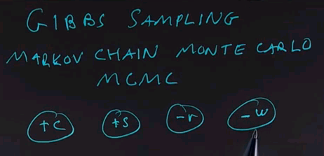
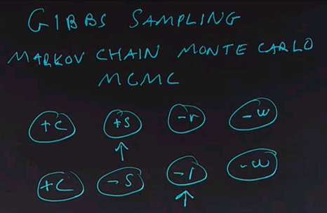
A technique called Gibbs sampling, named after the physicist Josiah Gibbs, takes all the evidence into account and not just the upstream evidence. It uses a method called Markov Chain Monte Carlo, or MCMC. The idea is that we resample just one variable at a time conditioned on all the others. That is, we have a set of variables, and we initialise them to random variables, keeping the evidence values fixed. Maybe we have values like this,
and that constitutes one sample, and now, at each iteration through the loop, we select just one non-evidence variable and resample it based on all the other variables. And that will give us another sample, and repeat that again.
Choose another variable. Resample that variable and repeat. We end up walking around in this space of assignments of variables randomly. Now, in rejection and likelihood sampling, each sample was independent of the other samples. In MCMC, that's not true. The samples are dependent on each other, and in fact, adjacent samples are very similar. They only vary or differ in one place. However, the technique is still consistent. We won't show the proof for that.
Monty Hall Problem
Now just one more thing. I can't help but describe what is probably the most famous probability problem of all. It's called the Monty Hall Problem after the game show host. And the idea is that you're on a game show, and there's 3 doors: door #1, door #2 and door #3. And behind each door is a prize, and you know that one of the doors contains an expensive sports car, which you would find desirable, and the other two doors contain a goat, which you would find less desirable.
Now, say you're given a choice, and let's say you choose door #1. But according to the conventions of the game, the host, Monty Hall, will now open one of the doors, knowing that the door that he opens contains a goat, and he shows you door #3. And he now gives you the opportunity to stick with your choice or to switch to the other door. What I want you to tell me is, what is your probability of winning if you stick to door #1, and what is the probability of winning if you switched to door #2?
The answer is that you have a 1/3 chance of winning if you stick with door #1 and a 2/3 chance if you switch to door #2. How do we explain that, and why isn't it 50/50? Well, it's true that there's two possibilities, but we've learned from probability that just because there are two options doesn't mean that both options are equally likely. It's easier to explain why the first door has a 1/3 probability because when you started, the car could be in any one of three places. You chose one of them. That probability was 1/3. And that probability hasn't been changed by the revealing of one of the other doors. Why is door #2 two-thirds? Well one way to explain it is that the probability has to sum to one, and if 1/3 is here, the 2/3 has to be here. But why doesn't the same argument that you use for one hold for two? Why can't we say the probability of two holding the car was 1/3 before this door was revealed? Why has that changed two and not changed one? And the reason is because we've learned something about door #2. We've learned that it wasn't the door that was flipped over by the host, and so that additional information has updated the probability, whereas we haven't learned anything additional about door #1 because it was never an option that the host might switch door #1. And in fact, in this case, if we reveal the door, we find that's where the car actually is. So you see, learning the probability may end up winning you something.
Monty Hall Letter
Now, as a final epilogue, I have here a copy of a letter written by Monty Hall himself in 1990 to Professor Lawrence Denenberg of Harvard who, with Harry Lewis, wrote a statistics book in which they used the Monty Hall Problem as an example, and they wrote to Monty asking him for permission to use his name. Monty kindly granted the permission, but in his letter, he writes, "As I see it, it wouldn't make any difference after the player has selected Door A, and having been shown Door C -- why should he then attempt to switch to Door B?" So, we see Monty Hall himself did not understand the Monty Hall Problem.
