AI class overview

This is an overview in point form of the content in the AI class.

Unit 1: Welcome to AI

Introduction

• Lots of work to do
• Will be ranked

Course Overview

Purpose of the class:

• To teach the basics of AI artificial intelligence
• To excite you

Structure:

• Videos -> Quizzes -> Answer Videos
• Assignments (like quizzes but without the answers) and exams

Intelligent Agents

• Agent has sensors to determine its environment
• Agent has actuators to affect its environment
• Agent interacts in a Perception-Action cycle
• Agent's Control Policy maps sensors to actuators

Applications of AI

• Finance
• Robotics
• Games
• Medicine
• Web
• Other fields

Terminology

• Fully Observable vs Partially Observable
  • Fully Observable environment: if what your agent can sense at any point in time is completely sufficient to make the optimal decision, i.e. if the sensors can see the entire state
  • Partially Observable environment: need memory in the agent to make the best possible decision, because the agents' sensors can't see the entire state
  • When we look at Hidden Markov Models we will learn more about structuring memory when state is partially observable
• Deterministic vs Stochastic
  • Deterministic environment: agent's actions uniquely determine the outcome, there is no randomness
  • Stochastic environment: outcome of actions involve a certain level of randomness
• Discrete vs Continuous
  • Discrete environment: finitely many states and actions
  • Continuous environment: infinitely many states and actions
• Benign vs Adversarial
  • Benign environments: not really out there to get you
  • Adversarial environments: harder to find good actions when your opponent is counteracting what you're trying to achieve

Checkers

• Fully observable
• Deterministic
• Discrete
• Adversarial

Poker

• Partially observable
• Stochastic
• Discrete
• Adversarial

Robot Car

• Partially observable
• Stochastic
• Continuous
• Benign

AI and Uncertainty

• AI is uncertainty management: what to do when you don't know what to do?
• Reasons for uncertainty:
  • Sensor limits
  • Stochastic environment
  • Laziness
  • Ignorance
  • Adversaries

Machine Translation

Google's translation system works probabilistically and the probabilities are inferred from known translations.

Summary

• Key applications of AI
• Intelligent agent
• 4 key attributes of environments
• Sources of uncertainty
• Rationality

Unit 2: Problem Solving

Introduction

• There are different types of problem with different approaches
  • Partially observable environments need special treatment which we will cover later

What is a Problem?

• Definition of a problem
  • Initial state
  • Actions(S) -> {a₁,a₂,a₃,...}
  • Result(S,a) -> S'
  • GoalTest(S) -> T|F
  • PathCost(S-a->S-a->S) -> n
    • StepCost(S,a,S') -> n

Example: Route Finding

• Categories of the state space:
  • Explored
  • Frontier
  • Unexplored

Tree Search

function TreeSearch( problem ):
  frontier = {[initial]}
  loop:
    if frontier is empty: return FAIL
    path = remove_choice( frontier )
    S = path.end
    if S is a goal: return path
    for a in actions:
      add [ path + a -> Result(S,a) ] to frontier

Graph Search

function GraphSearch( problem ):
  frontier = {[initial]}
  explored = {}
  loop:
    if frontier is empty: return FAIL
    path = remove_choice( frontier )
    S = path.end
    add S to explored
    if S is a goal: return path
    for a in actions:
      add [ path + a -> Result(S,a) ] to frontier
      unless Result(S,a) in frontier or explored

Breadth First Search

• always considers the shortest paths first
• goal test not applied when we add path to frontier
  • rather it's applied when we remove a path from the frontier
  • this is because the path might not be the best possible
  • can code up a custom BFS that checks upon insert into frontier and terminates early

Uniform Cost Search

• also known as Cheapest First Search
• is guaranteed to find the path with lowest total cost

Search Comparison

• Optimal: indicates that the algorithm will find a path and that path will be the "shortest" path
  • for Cheapest First that means the path with the lowest total cost
  • for Breadth First and Depth First the "shortest" path is the one with the least number of steps
• Complete: meaning if there is a goal somewhere the algorithm will find it

Algorithm	Optimal?	Complete?	Space
Breadth First Search	yes	yes	2n
Cheapest First Search (Uniform Cost)	yes	yes	~2n
Depth First Search	no	no	n

More on Uniform Cost Search

• Uniform Cost Search expands evenly in all directions from the initial state
• Greedy Best First Search expands using the shortest distance to the goal
• If there is a barrier Greedy Best First Search might find a longer than necessary path

A* Search

• A* could be called Best Estimated Total Path Cost First
• A* expands nodes with lowest f-values first
• f = g + h
• g(path) = path cost
• h(path) = h(S) = estimated distance to goal
• Whether A* finds the shortest path or not depends on the h-value
  • h must under-estimate to ensure shortest path is found

Optimistic Heuristics

• This argument applies to Tree Search
  • The argument for Graph Search is similar but more complicated
• When A* ends it returns a path cost c with a zero estimated cost (h) and a cost representing the total actual cost (g)
  • We know that all other paths on the frontier have an estimated cost that's greater than c because the frontier is explored in cheapest first order
  • If h is optimistic then the estimated cost is less than the true cost, so the path p must have a cost that's less than the true cost of any other paths on the frontier
    • Further, any paths that go beyond the frontier must have a cost that's greater still because we agreed that the step cost is always >= 0

State Space

• The State Space represents the state of the agent and the state of the environment
• We need efficient algorithms for searching through state spaces because the number of combinations of state variables becomes large very quickly

Sliding Blocks Puzzle

• The sliding blocks puzzle, also known as the 15 puzzle, can be solved using search techniques
• The goal state has each number 1 to 15 in order from left to right, top to bottom
• Admissible A* heuristic functions
  • h₁: the number of misplaced blocks
  • h₂: the sum of the distances that each block would have to move to get to the right position
• h₂ causes A* to expand fewer paths than h₁ because it is always greater than or equal to h₁
• Heuristics can be derived from a simple mechanical manipulation of the formal description of the problem
  • crossing out parts of the rules like this is called generating a relaxed problem
  • adding new operators only makes the problem easier, and thus never overestimates, and thus is admissible
• Another way to come with a good heuristic is to say that a new heuristic h is equal to the maximum of h₁ and h₂
  • that's guaranteed to be admissible as long as h₁ and h₂ are admissible, because it still never overestimates
  • and it's guaranteed to be better, because it's getting closer to the true value
• The only problem with combining multiple heuristics like this is that there is some cost to compute the heuristic, and it could take longer to compute even if we end up expanding fewer paths

Problems with Search

• Search based problem solving works when:
  • The domain is fully observable; we must be able to see what initial state we are in
  • The domain must be known; that is, we have to know the set of actions available to us
  • The domain must be discrete; there must be a finite number of actions to choose from
  • The domain must be deterministic; we have to know the result of taking an action
  • The domain must be static; there must be nothing else in the world that can change the world except our own actions
• If all of the above conditions are true we can search for a plan which solves the problem and is guaranteed to work

A Note on Implementation

• The implementation of a 'path' is called a 'node'
• Nodes are data-structures with four fields:
  • The state field indicates the state at the end of the path
  • The action was the action it took to get there
  • The cost is the total cost
  • And the parent is a pointer to another node
• So we have a linked list of nodes representing a path
  • we'll use the word "path" for the abstract idea
  • and the word "node" for the representation in the computer memory
• there are two main data structures that deal with nodes:
  • the frontier
    • in the frontier the operations we have to deal with are removing the best item from the frontier and adding in the new ones
      • this suggests we should implement it as a priority queue, which knows how to keep track of the best items in proper order
    • but, we also need to have an additional operation of a membership test, is a new item in the frontier?, and that suggests representing it as a set, which can be built from a hashtable or a tree
      • the most efficient implementations of search actually have both representations
  • the explored list
    • all we have to do there is be able to add new members and check for membership
      • so we represent that as a single set, which again can be done with either a hashtable or a tree

Unit 3: Probability in AI

Introduction

• This unit is concerned with structured probabilities using Bayes Networks
• This unit is important: Bayes Networks are used extensively in almost all fields of smart computer systems
• A Bayes Network enables you to reason from observable variables to hidden causes
• A Bayes Network is composed of nodes
  • Nodes correspond to events, or random variables, that you may or may not know
  • Nodes are linked by arcs
    • Arcs suggest that the child of an arc is influenced by its parent in a probabilistic way
• We will assume binary (and therefore discrete) variables for this unit
• A Bayes Network with 16 nodes specifies a probability distribution of 2¹⁶ values
• A Bayes Network is a compact representation of a distribution over typically very very large joint probability distributions of all the variables
• We will learn about the following related to Bayes Networks:
  • Binary Events
  • Probability
  • Simple Bayes Networks
  • Conditional Independence
  • Bayes Networks
  • D-separation
  • Parameter Counts
• Bayes Networks are also the building blocks of more advanced AI techniques such as:
  • Particle filters
  • Hidden Markov Models
  • MDPs
  • POMDPs
  • Kalman filters
  • Many others...

Probability/Coin Flip

• Probabilities are the corner stone of artificial intelligence
• Probabilities are used to express uncertainty, and managing uncertainty is key to many AI problems
• In a coin toss if the probability of heads (H) is P(H)=1/2 then the probability of not heads (i.e. tails) is:
  • P(¬H) = P(T) = 1 - P(H) = 1 - 1/2 = 1/2
• In a loaded coin toss if the probability of heads (H) is P(H)=1/4 then the probability of not heads (i.e. tails) is:
  • P(¬H) = P(T) = 1 - P(H) = 1 - 1/4 = 3/4
• In three successive independent coin tosses, the probability of the coin coming up heads all three times is P(H,H,H) = P(H)*P(H)*P(H) = P(H)³ = (1/2)³ = 1/8
  • Note: we can multiply the probabilities because the coin tosses are independent events
• If we flip a coin four times, and call X_i the result of the i^th coin flip, the probability that all four flips render the same result, either all heads or all tails, is:
  • P(H,H,H,H) = P(H)⁴ = (1/2)⁴ = 1/16
• Similarly:
  • P(T,T,T,T) = P(T)⁴ = (1/2)⁴ = 1/16
• The probability of either one occurring is:
  • P(H,H,H,H) + P(T,T,T,T) = 1/16 + 1/16 = 1/8
• If we flip a coin 4 times, the probability that within the set {X₁,X₂,X₃,X₄} there are at least 3 (or more) heads is 5/16 as calculated from the following table:

Combination	3 or more heads?
HHHH	yes
HHHT	yes
HHTH	yes
HHTT
HTHH	yes
HTHT
HTTH
HTTT
THHH	yes
THHT
THTH
THTT
TTHH
TTHT
TTTH
TTTT

Probability Summary

• If an event has a certain probability, P, then the complementary event has probability 1-P
• Independence notation:
  • X⊥Y
• Joint probability:
  • P(X,Y)
• Marginals:
  • P(X) and P(Y)
• Joint probability of independent events is multiplication of the marginals:
  • P(X,Y) = P(X)P(Y)

Dependence

• As an example of dependence consider two coin flips, wherein the result of the flip of the first coin determines which coin you flip next
• P(X₁=H) = 1/2:
  • X₁=H: P(X₂=H|X₁=H) = 0.9
  • X₁=T: P(X₂=H|X₁=T) = 0.2

P(X2=H)
  = P(X2=H|X1=H)P(X1=H) +
    P(X2=H|X1=T)P(X1=T)
  = 0.9 * 1/2 + 0.2 * 1/2
  = 0.45 + 0.1
  = 0.55

What We Learned

• Total probability:
  • $P(Y)=\sum _{i}P(Y|X=i)\cdot P(X=i)$
• Negation of probabilities:
  • $P(\lnot X|Y)=1-P(X|Y)$

Weather

• Given:
  • P(D₁=sunny) = 0.9
  • P(D₂=sunny|D₁=sunny) = 0.8
• We can derive by negation:
  • P(D₁=rainy) = 0.1
  • P(D₂=rainy|D₁=sunny) = 0.2
• Given:
  • P(D₂=sunny|D₁=rainy) = 0.6
• We can derive by negation:
  • P(D₂=rainy|D₁=rainy) = 0.4
• What is the probability that D₂ is sunny?

P(D2=sunny)
  = P(D2=sunny|D1=sunny)P(D1=sunny) +
    P(D2=sunny|D1=rainy)P(D1=rainy)
  = 0.8 * 0.9 + 0.6 * 0.1
  = 0.72 + 0.06
  = 0.78

• From which we can derive by negation:
  • P(D₂=rainy) = 1 - P(D₂=sunny) = 1 - 0.78 = 0.22
• What is the probability that D₃ is sunny?

P(D3=sunny)
  = P(D3=sunny|D2=sunny)P(D2=sunny) +
    P(D3=sunny|D2=rainy)P(D2=rainy)
  = 0.8 * 0.78 + 0.6 * 0.22
  = 0.624 + 0.132
  = 0.756

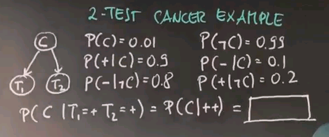
Cancer

• Find P(C|+), the probability of cancer given a positive test
• Given the prior:
  • P(C) = 0.01
• We can derive by negation:
  • P(¬C) = 1 - P(C) = 0.99
• Given:
  • P(+|C) = 0.9
• We can derive by negation:
  • P(-|C) = 1 - P(+|C) = 0.1
• Given:
  • P(+|¬C) = 0.2
• We can derive by negation:
  • P(-|¬C) = 1 - P(+|¬C) = 0.8
• Using the product rule P(A,B) = P(A|B)P(B) we can calculate:
  • P(+,C) = P(+|C)P(C) = 0.9 * 0.01 = 0.009
  • P(-,C) = P(-|C)P(C) = 0.1 * 0.01 = 0.001
  • P(+|¬C) = P(+|¬C)P(¬C) = 0.2 * 0.99 = 0.198
  • P(-,¬C) = P(-|¬C)P(¬C) = 0.8 * 0.99 = 0.792
• P(+) is the total probability:
  • P(+|C)P(C) + P(+|¬C)P(¬C) =
  • 0.9 * 0.01 + 0.2 * 0.99 = 0.207
• Now P(+,C) = P(C,+), meaning we can expand with the product rule:
  • P(C|+)P(+) = P(+|C)P(C)
• To get Bayes Rule:
  • P(C|+) = P(+|C)P(C)/P(+)
    • Posterior: P(C|+)
    • Likelihood: P(+|C)
    • Prior: P(C)
    • Marginal likelihood: P(+)
• Substituting from the above:
  • P(C|+) = 0.9 * 0.01 / 0.207
  • P(C|+) = 0.0435

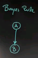
Bayes Rule

• $P(A|B)={\frac {P(B|A)P(A)}{P(B)}}$
  • P(A|B): posterior
  • P(B|A): likelihood
  • P(A): prior
  • P(B): marginal likelihood
• $P(B)=\sum _{a}P(B|A=a)\cdot P(A=a)$
  • The probability of the evidence, known as the marginal likelihood, P(B), is the total probability

Bayes Network

• Observability:
  • A: not observable
  • B: observable
• 3 parameters for this Bayes Network:
  • P(A)
  • P(B|A)
  • P(B|¬A)
• Diagnostic Reasoning (observations to causes):
  • P(A|B)
  • P(A|¬B)

Computing Bayes Rule

• $P(A|B)+P(\lnot A|B)=1$
• $P(A|B)={\frac {P(B|A)\cdot P(A)}{P(B)}}$
• $P(\lnot A|B)={\frac {P(B|\lnot A)\cdot P(\lnot A)}{P(B)}}$
• $P'(A|B)=P(B|A)\cdot P(A)$
• $P'(\lnot A|B)=P(B|\lnot A)\cdot P(\lnot A)$
• $P(A|B)=\eta \cdot P'(A|B)$
• $P(\lnot A|B)=\eta \cdot P'(\lnot A|B)$
• $\eta =(P'(A|B)+P'(\lnot A|B))^{-1}$

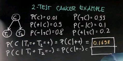
Two Test Cancer

	prior	+	+	P'	P(C|++)
C	0.01	0.9	0.9	0.0081	0.1698
¬C	0.99	0.2	0.2	0.0396	0.8301
				0.0477

	prior	+	-	P'	P(C|+-)
C	0.01	0.9	0.1	0.0009	0.0056
¬C	0.99	0.2	0.8	0.1584	0.9943
				0.1593

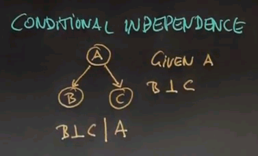
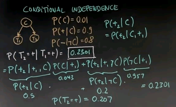
Conditional Independence

• B⊥C|A
  • does not imply B⊥C

• Due to conditional independence P(+₂|C,+₁) = P(+₂|C)
• Note that the first test has 20% change of being positive, whereas the second test has a 23% chance of being positive, given that our first test was positive

Absolute and Conditional

• B⊥C does not imply B⊥C|A
• B⊥C|A does not imply B⊥C

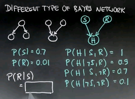
Confounding Cause

• Here we see two causal variables confounded in a single observation variable. That is sunny (S) and raise (R) influence happiness (H).
• The probability of P(R|S) = P(R) because S and R are absolutely independent.

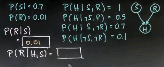
Explaining Away

• Given that it's sunny and I'm happy I can explain my happiness due to sunniness so that makes a raise less likely
• Given that it's not sunny and I'm happy I can explain my happiness due to a raise so that makes a raise more likely
• We can use Bayes Theorem to factor P(R|H,S) as:
  • $P(R|H,S)={\frac {P(H|R,S)\cdot P(R|S)}{P(H|S)}}$
• We know the following due to absolute independence:
  • $P(R|S)=P(R)$
• We can compute P(H|S) using total probability:
  • Failed to parse (syntax error): {\displaystyle P(H|S) = P(H|R,S)P(R) + P(H|¬R,S)P(¬R)}
• We can substitute into Bayes Theorm as follows:
  • Failed to parse (syntax error): {\displaystyle P(R|H,S)=\frac{P(H|R,S) \cdot P(R)}{P(H|R,S)P(R) + P(H|¬R,S)P(¬R)}}
• Then we can compute:
  • ${\frac {1\cdot 0.01}{1\cdot 0.01+0.7\cdot 0.99}}=0.0142$